
The following problem appeared in an assignment in the Princeton course COS 126 . The problem description is taken from the course itself.
Recursive Graphics
Write a program that plots a Sierpinski triangle, as illustrated below. Then develop a program that plots a recursive patterns of your own design.
 https://sandipanweb.files.wordpress.com/2018/01/sierpinski91.png?w=150 150w, https://sandipanweb.files.wordpress.com/2018/01/sierpinski91.png?w=300 300w, https://sandipanweb.files.wordpress.com/2018/01/sierpinski91.png?w=768 768w, https://sandipanweb.files.wordpress.com/2018/01/sierpinski91.png?w=… 1024w, https://sandipanweb.files.wordpress.com/2018/01/sierpinski91.png 1179w” sizes=”(max-width: 676px) 100vw, 676px” />
Part 1.
The Sierpinski triangle is an example of a fractal pattern. The pattern was described by Polish mathematician Waclaw Sierpinski in 1915, but has appeared in Italian art since the 13th century. Though the Sierpinski triangle looks complex, it can be generated with a short recursive program.
Examples. Below are the target Sierpinski triangles for different values of order N.
 https://sandipanweb.files.wordpress.com/2018/01/sierpinski21.png?w=133 133w, https://sandipanweb.files.wordpress.com/2018/01/sierpinski21.png?w=265 265w” sizes=”(max-width: 564px) 100vw, 564px” />
Our task is to implement a recursive function sierpinski(). We need to think recursively: our function should draw one black triangle (pointed downwards) and then call itself recursively 3 times (with an appropriate stopping condition). When writing our program, we should exercise modular design.
The following code shows an implementation:
class Sierpinski:
# Height of an equilateral triangle whose sides are of the specified length.
def height(self, length):
return sqrt(3) * length / 2.# Draws a filled equilateral triangle whose bottom vertex is (x, y)
# of the specified side length.
def filledTriangle(self, x, y, length):
h = self.height(length)
draw(np.array([x, x+length/2., x-length/2.]), np.array([y, y+h, y+h]), alpha=1)# Draws an empty equilateral triangle whose bottom vertex is (x, y)
# of the specified side length.
def emptyTriangle(self, x, y, length):
h = self.height(length)
draw(np.array([x, x+length, x-length]), np.array([y+2*h, y, y]), alpha=0)# Draws a Sierpinski triangle of order n, such that the largest filled
# triangle has bottom vertex (x, y) and sides of the specified length.
def sierpinski(self, n, x, y, length):
self.filledTriangle(x, y, length)
if n > 1:
self.sierpinski(n-1, x-length/2., y, length/2.)
self.sierpinski(n-1, x+length/2., y, length/2.)
self.sierpinski(n-1, x, y+self.height(length), length/2.)
The following animation shows how such a triangle of order 5 is drawn recursively.
The following animation shows how such a triangle of order 6 is drawn recursively.
A diversion: fractal dimension.
Formally, we can define the Hausdorff dimension or similarity dimension of a self-similar figure by partitioning the figure into a number of self-similar pieces of smaller size. We define the dimension to be the log (# self similar pieces) / log (scaling factor in each spatial direction). For example, we can decompose the unit square into 4 smaller squares, each of side length 1/2; or we can decompose it into 25 squares, each of side length 1/5. Here, the number of self-similar pieces is 4 (or 25) and the scaling factor is 2 (or 5). Thus, the dimension of a square is 2 since log (4) / log(2) = log (25) / log (5) = 2. We can decompose the unit cube into 8 cubes, each of side length 1/2; or we can decompose it into 125 cubes, each of side length 1/5. Therefore, the dimension of a cube is log(8) / log (2) = log(125) / log(5) = 3.
We can also apply this definition directly to the (set of white points in) Sierpinski triangle. We can decompose the unit Sierpinski triangle into 3 Sierpinski triangles, each of side length 1/2. Thus, the dimension of a Sierpinski triangle is log (3) / log (2) ≈ 1.585. Its dimension is fractional—more than a line segment, but less than a square! With Euclidean geometry, the dimension is always an integer; with fractal geometry, it can be something in between. Fractals are similar to many physical objects; for example, the coastline of Britain resembles a fractal, and its fractal dimension has been measured to be approximately 1.25.
Part 2.
Drawing a tree recursively, as described here:
 https://sandipanweb.files.wordpress.com/2018/01/treed.png?w=150 150w, https://sandipanweb.files.wordpress.com/2018/01/treed.png?w=300 300w, https://sandipanweb.files.wordpress.com/2018/01/treed.png 708w” sizes=”(max-width: 629px) 100vw, 629px” />
The following shows how a tree of order 10 is drawn:
The next problem appeared in an assignment in the Cornell course CS1114 . The problem description is taken from the course itself.
Bilinear Interpolation
Let’s consider a 2D matrix of values at integer grid locations (e.g., a grayscale image). To interpolate values on a 2D grid, we can use the 2D analogue of linear interpolation: bilinear interpolation. In this case, there are four neighbors for each possible point we’d like to interpolation, and the intensity values of these four neighbors are all combined to compute the interpolated intensity, as shown in the next figure.
 https://sandipanweb.files.wordpress.com/2018/01/f6.png?w=150 150w, https://sandipanweb.files.wordpress.com/2018/01/f6.png?w=300 300w, https://sandipanweb.files.wordpress.com/2018/01/f6.png?w=768 768w, https://sandipanweb.files.wordpress.com/2018/01/f6.png?w=1024 1024w, https://sandipanweb.files.wordpress.com/2018/01/f6.png 1030w” sizes=”(max-width: 676px) 100vw, 676px” />
In the figure, the Q values represent intensities. To combine these intensities, we perform linear interpolation in multiple directions: we first interpolate in the x direction (to get the value at the blue points), then in the y direction (to get the value at the green points).
Image transformations
Next, we’ll use the interpolation function to help us implement image transformations.
A 2D affine transformation can be represented with a 3 ×3 matrix T:
 https://sandipanweb.files.wordpress.com/2018/01/f4.png?w=150 150w” sizes=”(max-width: 194px) 100vw, 194px” />
Recall that the reason why this matrix is 3×3, rather than 2 ×2, is that we operate in homogeneous coordinates; that is, we add an extra 1 on the end of our 2D coordinates (i.e., (x,y) becomes (x,y,1)), in order to represent translations with a matrix multiplication. To apply a transformation T to a pixel, we multiply T by the pixel’s location:
 https://sandipanweb.files.wordpress.com/2018/01/f5.png?w=150 150w, https://sandipanweb.files.wordpress.com/2018/01/f5.png?w=300 300w” sizes=”(max-width: 486px) 100vw, 486px” />
The following figure shows a few such transformation matrices:
 https://sandipanweb.files.wordpress.com/2018/01/f8.png?w=1086&h… 1086w, https://sandipanweb.files.wordpress.com/2018/01/f8.png?w=119&h=150 119w, https://sandipanweb.files.wordpress.com/2018/01/f8.png?w=238&h=300 238w, https://sandipanweb.files.wordpress.com/2018/01/f8.png?w=768&h=966 768w, https://sandipanweb.files.wordpress.com/2018/01/f8.png?w=814&h=… 814w” sizes=”(max-width: 543px) 100vw, 543px” />
To apply a transformation T to an entire image I, we could apply the transformation to each of I’s pixels to map them to the output image. However, this forward warpingprocedure has several problems. Instead, we’ll use inverse mapping to warp the pixels of the output image back to the input image. Because this won’t necessarily hit an integer-valued location, we’ll need to use the (bi-linear) interpolation to determine the intensity of the input image at the desired location, as shown in the next figure.
 https://sandipanweb.files.wordpress.com/2018/01/f7.png?w=150&h=82 150w, https://sandipanweb.files.wordpress.com/2018/01/f7.png?w=300&h=164 300w, https://sandipanweb.files.wordpress.com/2018/01/f7.png?w=768&h=419 768w, https://sandipanweb.files.wordpress.com/2018/01/f7.png 905w” sizes=”(max-width: 516px) 100vw, 516px” />
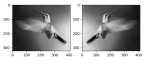
To demo the transformation function, let’s implement the following on a gray scale bird image:
1. Horizontal flipping
 https://sandipanweb.files.wordpress.com/2018/01/out_flip1.png?w=150 150w, https://sandipanweb.files.wordpress.com/2018/01/out_flip1.png?w=300 300w” sizes=”(max-width: 579px) 100vw, 579px” />
2. Scaling by a factor of 0.5
 https://sandipanweb.files.wordpress.com/2018/01/out_scale.png?w=150 150w, https://sandipanweb.files.wordpress.com/2018/01/out_scale.png?w=300 300w” sizes=”(max-width: 510px) 100vw, 510px” />
3. Rotation by 45 degrees around the center of the image
 https://sandipanweb.files.wordpress.com/2018/01/out_rot1.png?w=150 150w, https://sandipanweb.files.wordpress.com/2018/01/out_rot1.png?w=300 300w” sizes=”(max-width: 567px) 100vw, 567px” />
The next animations show rotation and sheer transformations with the Lena image:


Next, let’s implement a function to transform RGB images. To do this, we need to simply call transform image three times, once for each channel, then put the results together into a single image. Next figures and animations show some results on an RGB image.
Some non-linear transformations
The next figure shows the transform functions from here:
 https://sandipanweb.files.wordpress.com/2018/01/f9.png?w=150 150w, https://sandipanweb.files.wordpress.com/2018/01/f9.png?w=300 300w, https://sandipanweb.files.wordpress.com/2018/01/f9.png 677w” sizes=”(max-width: 676px) 100vw, 676px” />
The next figures and animations show the application of the above non-linear transforms on the Lena image.
Wave1
 https://sandipanweb.files.wordpress.com/2018/01/out_f1.png?w=150 150w, https://sandipanweb.files.wordpress.com/2018/01/out_f1.png?w=300 300w” sizes=”(max-width: 568px) 100vw, 568px” />
Wave2
 https://sandipanweb.files.wordpress.com/2018/01/out_f2.png?w=150 150w, https://sandipanweb.files.wordpress.com/2018/01/out_f2.png?w=300 300w” sizes=”(max-width: 640px) 100vw, 640px” />
Swirl
 https://sandipanweb.files.wordpress.com/2018/01/out_swirl.png?w=150 150w, https://sandipanweb.files.wordpress.com/2018/01/out_swirl.png?w=300 300w” sizes=”(max-width: 595px) 100vw, 595px” />
Warp
 https://sandipanweb.files.wordpress.com/2018/01/out_warp.png?w=150 150w, https://sandipanweb.files.wordpress.com/2018/01/out_warp.png?w=300 300w” sizes=”(max-width: 607px) 100vw, 607px” />
Some more non-linear transforms:

Anti-aliasing
There is a problem with our interpolation method above: it is not very good at shrinking images, due to aliasing. For instance, if let’s try to down-sample the following bricks image by a factor of 0.4, we get the image shown in the following figure: notice the strange banding effects in the output image.
Original Image
 https://sandipanweb.files.wordpress.com/2018/01/bricks_gray.png?w=1… 123w, https://sandipanweb.files.wordpress.com/2018/01/bricks_gray.png?w=2… 247w” sizes=”(max-width: 542px) 100vw, 542px” />
Down-sampled Image with Bilinear Interpolation
 https://sandipanweb.files.wordpress.com/2018/01/out_scale_b1.png?w=… 123w” sizes=”(max-width: 542px) 100vw, 542px” />
The problem is that a single pixel in the output image corresponds to about 2.8 pixels in the input image, but we are sampling the value of a single pixel—we should really be averaging over a small area.
To overcome this problem, we will create a data structure that will let us (approximately) average over any possible square regions of pixels in the input image: an image stack. An image stack is a 3D matrix that we can think of as, not surprisingly, a stack of images, one on top of the other. The top image in the cube will be the original input image. Images further down the stack will be the input image with progressively larger amounts of blur. The size of the matrix will be rows × cols × num levels, where the original (grayscale) image has size rows×cols and there are num levels images in the stack.
Before we use the stack, we must write a function to create it, which takes as input a (grayscale) image and a number of levels in the stack, and returns a 3D matrix stack corresponding to the stack. Again, the first image on the stack will be the original image. Every other image in the stack will be a blurred version of the previous image. A good blur kernel to use is:
 https://sandipanweb.files.wordpress.com/2018/01/f10.png?w=150 150w” sizes=”(max-width: 186px) 100vw, 186px” />
Now, for image k in the stack, we know that every pixel is a (weighted) average of some number of pixels (a k × k patch, roughly speaking) in the input image. Thus, if we down-sample the image by a factor of k, we want to sample pixels from level k of the stack.
⇒ Let’s write the following function to create image stack that takes a grayscale image and a number max levels, and returns an image stack.
from scipy import signal
def create_image_stack(img, max_level):
K = np.ones((3,3)) / 9.
image_stack = np.zeros((img.shape[0], img.shape[1], max_level))
image_stack[:,:,0] = img
for l in range(1, max_level):
image_stack[:,:,l] = signal.convolve2d(image_stack[:,:,l-1], K,
boundary=’symm’, mode=’same’)
return image_stack
The next animation shows the image stack created from the bricks image.
Trilinear Interpolation
Now, what happens if we down-sample the image by a fractional factor, such as 3.6? Unfortunately, there is no level 3.6 of the stack. Fortunately, we have a tool to solve this problem: interpolation. We now potentially need to sample a value at position (row,col,k) of the image stack, where all three coordinates are fractional. We therefore something more powerful than bilinear interpolation: trilinear interpolation! Each position we want to sample now has eight neighbors, and we’ll combine all of their values together in a weighted sum.
This sounds complicated, but we can write this in terms of our existing functions. In particular, we now interpolate separately along different dimensions: trilinear interpolation can be implemented with two calls to bilinear interpolation and one call to linear interpolation.
Let’s implement a function trilerp like the following that takes an image stack, and a row, column, and stack level k, and returns the interpolated value.
def trilerp (img_stack, x, y, k):
if k < 1: k = 1
if k == int(k):
return bilerp(img_stack[:,:,k-1], x, y)
else:
f_k, c_k = int(floor(k)), int(ceil(k))
v_f_k = bilerp(img_stack[:,:,f_k-1], x, y)
v_c_k = bilerp(img_stack[:,:,c_k-1], x, y)
return linterp(k, f_k, c_k, v_f_k, v_c_k)
Now we can finally implement a transformation function that does proper anti-aliasing. In order to do this, let’s implement a function that will
- First compute the image stack.
- Then compute, for the transformation T, how much T is scaling down the image. If T is defined by the six values a,b,c,d,e,f above, then, to a first approximation, the downscale factor is:
 https://sandipanweb.files.wordpress.com/2018/01/f11.png?w=150 150w” sizes=”(max-width: 251px) 100vw, 251px” />
However, if k < 1 (corresponding to scaling up the image), we still want to sample from level 1. This situation reverts to normal bilinear interpolation. - Next call the trilerp function on the image stack, instead of bilerp on the input image.

The next figure shows the output image obtained image transformation with proper anti-aliasing:
Down-sampled Image with Anti-aliasing using Trilinear Interpolation https://sandipanweb.files.wordpress.com/2018/01/out_scale_t.png?w=1… 120w” sizes=”(max-width: 505px) 100vw, 505px” />
As we can see from the above output, the aliasing artifact has disappeared.
The same results are obtained on the color image, as shown below, by applying the trilerp function on the color channels separately and creating separate image stacks for different color channels.
Original Image
 https://sandipanweb.files.wordpress.com/2018/01/bricks_rgb.png?w=12… 123w, https://sandipanweb.files.wordpress.com/2018/01/bricks_rgb.png?w=24… 247w” sizes=”(max-width: 414px) 100vw, 414px” />
Down-sampled Image with Bilinear Interpolation
 https://sandipanweb.files.wordpress.com/2018/01/out_scale_b2.png?w=… 120w” sizes=”(max-width: 412px) 100vw, 412px” />
Down-sampled Image with Anti-aliasing
 https://sandipanweb.files.wordpress.com/2018/01/out_scale_t1.png?w=… 123w” sizes=”(max-width: 412px) 100vw, 412px” />