Introduction

Hybrid Quantum-Classical Computing (HQCC) (a.k.a. Variational Quantum Eigensolver (VQE)) is often touted as one of the main algorithms of Quantum AI. In fact, Rigetti, a Silicon Valley company which for several years has provided cloud access to their superconductive quantum computer, has designed its services around the HQCC paradigm.

In this brief blog post, I will explain how HQCC can be understood in terms of quantum Bayesian networks. In the process, I will review some basic facts about classical and quantum Bayesian networks (bnets).

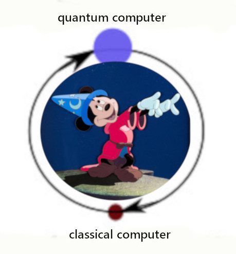
HQCC is often symbolized by a feedback loop between a quantum computer and a classical computer.

Classical Bayesian Networks

First, let’s review some basic facts about classical bnets.

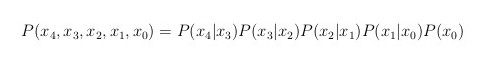
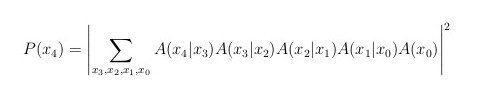
Consider the chain rule for conditional probabilities. For the case of a probability distribution P() that depends on 5 random variables x₀, x₁, …, x₄, one has

This last equation can be represented graphically by the following bnet, a “fully connected” DAG (Directed Acyclic Graph) in which an arrow points into x_j from all its predecessors x_j-1, x_j-2,…, x₁, x₀ for j=1, 2, …,4:

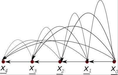
For definiteness, we have chosen the number of nodes nn=5. How to generalize this so that nn equals any integer greater than 1 is obvious.

Henceforth, we will represent a random variable by an underlined letter and the values it assumes by a letter that is not underlined. For instance, x= x.

Mathematicians often represent a random variable by an upper case letter and the values it assumes by a lower case letter. For instance, X= x. For a physicist like me, that convention is not very convenient because physicists use upper case letters to mean all sorts of things that aren’t random variables. Likewise, they often want to use a lower case letter for a random variable. For this reason, I personally find the upper case letter convention for denoting random variables too burdensome. That is why I use the underlined letter convention instead.

Mathematicians have a rigorous definition for a random variable, but for the purposes of this blog post, a random variable is just the name given to a node of a bnet. This will be true for both classical and quantum bnets.

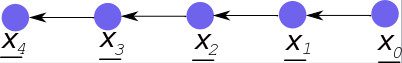
The arrows in a bnet denote dependencies. The fully connected bnet given above contains all possible dependencies. When each node depends only on its immediate predecessor, we get what is called a Markov chain. The Markov chain with nn=5 is:

bnets are technically acyclic graphs, so feedback loops are forbidden. However, as long as you understand that the following diagram should be “unrolled” into a Markov chain in which there are 2 types of nodes (the ones with an even subscript and the ones with an odd subscript), one can represent this special type of Markov chain with two types of nodes by the following diagram, where j=0, 1, …, nn-1:

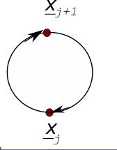
This last diagram is a special case of what is called in the business, a dynamical Bayesian network (DBN). An early type of DBN that you might already be familiar with is the famous Kalman filter.

Note that in this brief intro to classical bnets, we have only used discrete nodes with a discrete random variable x_j for j=0, 1, 2, …, nn-1. However, any one of those nodes can be easily replaced by a continuous node with a continuous random variable x_j. A continuous node x_j has a probability density instead of a probability distribution as its transition matrix P(x_j| parents of x_j), and one integrates rather than sums over its states x_j.

The definition of classical bnets is very simple. In the final analysis, bnets are just a graphical way to display the chain rule for conditional probabilities. It’s a simple but extremely productive definition. Classical bnets remind me of another simple but extremely productive definition, that of a Group in Mathematics. To paraphrase the bard Christopher Marlowe, the definition of a Group (and that of a bnet) is the definition that launched a thousand profound theorems.

Quantum Bayesian Networks

Next, we will review some basic facts about quantum bnets.

A brief history of quantum bnets: The first paper about quantum bnets was this one by me. In that paper, quantum bnets are used to represent pure states only. In subsequent papers, for instance, this one, I explained how to use quantum bnets to represent mixed states too. Quantum bnets led me to the invention of the definition of squashed entanglement.

Born’s Rule says that in Quantum Mechanics, one gets a probability P by taking the absolute value squared of a complex-valued “probability amplitude” A. In other words, P=|A|².

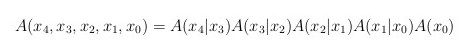
To define a quantum bnet, we write a chain rule for conditional probability amplitudes (A’s instead of P’s). For example, for nn=5, one has

This chain rule can be represented by the same diagram that we used above to represent the fully connected nn=5 classical bnet. However, note that now
node x_j has a complex-valued transition matrix A(x_j|parents of x_j) instead of a real-valued one P(x_j|parents of x_j). For that reason, henceforth, we will represent quantum nodes by a fluffy blue ball instead of the small brown balls that we have been using to represent classical nodes.

Just like we defined Markov chains for classical bnets, one can define them for quantum bnets. In both cases, every node depends only on its immediate predecessor. For a quantum Markov chain with nn=5, one has

which can be represented by the following quantum bnet:

It’s important to stress that quantum bnets have always, from the very beginning, been intended merely as a graphical way to represent the state vectors of quantum mechanics. They do not add any new constraints to the standard axioms of quantum mechanics. Furthermore, they are not intended to be a new interpretation of quantum mechanics.

Coherent and Incoherent sums

In this section, we will consider coherent and incoherent sums of quantum bnets. For simplicity, we will restrict the discussion of this section to quantum Markov chains, but everything we say in this section can be easily generalized to an arbitrary quantum bnet, including the fully connected one.

Suppose we have a classical Markov chain with nodes x₀, x₁, …, x₄ and we want to calculate the probability distribution P(x₄) of its last node. One does so by summing over all nodes except the last one:

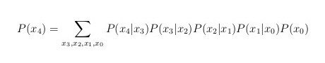
This last equation can be rewritten in terms of amplitudes in the equivalent form:

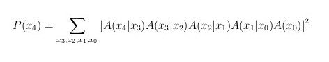
In the classical case above, we sum over all the variables outside the magnitude squared. A sum over a variable that is placed outside the absolute value squared will be called an incoherent sum. But the axioms of quantum mechanics also allow and give a meaning to, sums of variables that are placed inside the magnitude squared. A sum over a variable that is placed inside the absolute value squared will be called a coherent sum. For example, in the last equation, if we replace all the incoherent sums by coherent ones, we get:

But that’s not the whole story. One does not have to sum over all variables in an incoherent way or over all variables in a coherent way. One can sum over some variables coherently and over others incoherently. For example, one might be interested in the following sums:

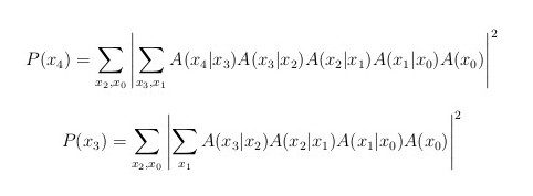
(Footnote: The quantities called P(x₄) and P(x₃) in the equations of this section might require normalization before they are true probability distributions.)

Quantum Bayesian Network point of view

The last 2 equations can be represent using dynamical quantum bnets, as follows:

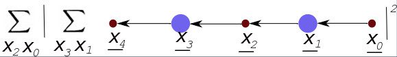
and

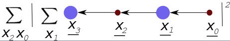
(Footnote: One can also consider 2 diagrams like the last 2 diagrams, but with

• coherent sums of the x_j with j even (instead of odd) and
• incoherent sums of the x_j with j odd (instead of even).

Also, nn itself is usually very large to allow convergence to an equilibrium distribution of P(x_nn-1) and P(x_nn-2), and nn can be either odd or even.)

The graphical part of the last two diagrams can be represented by the following feedback loop:

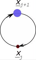
This last feedback loop is equivalent to the feedback loop with the Fantasia cartoon of Mickey Mouse that we started this blog post with and that we described as a pictorial representation of HQCC.