

Picture Courtesy: Freepik
The article explains the algorithm behind the recently introduced Python package named PyHard, based on the concept of Instance Space Analysis. It helps in assessing the quality of a dataset and identifying what are the instances which are hard/easy to classify. With the help of this algorithm we can separate out noisy instances. It also provides an interactive visualization tool to deep dive into the instance space.
Motivation:
Many a times, during a classification exercise, we think that is there any easier way to know which are the observations in my dataset which is bringing my accuracy down? or what are the regions in a dataset where any algorithm is expected to perform well?. I also had similar thought when I was browsing casually through the latest arXiv papers and it is exactly when the paper on PyHard caught my eyes. Here, I will try to explain the concept in a simple language.
Summary:
The paper explains a way to understand and visualize which are the observations, difficult to classify by any algorithm and which are the easier ones. The authors also propose a method to assess the overall quality of a dataset and how a classification model will perform on it. They also provide a complete visualization App to visualize the instance space in different ways, interact with it and draw insight. The full paper can be found in the link https://arxiv.org/abs/2109.14430 authored by Pedro Yuri Arbs Paiva, Kate Smith-Miles, Maria G. Valeriano and Ana Carolina Lorena.
Method:
The algorithm is built on Instant Space Analysis (ISA), a method to predict the performance of ML models in terms of meta-features, a set of hardness measures (explained later), of multiple public datasets. This is done by combining meta-features and model performance in a new embedding, mapping high dimensional meta-features into a 2-D space by solving optimization problem so that it displays as much of linear trend as possible and plotting the embedding for visual inspection. To understand the hardness of instances within a single dataset, in PyHard, a similar concept is applied. The picture below describes the ISA framework on a single dataset.
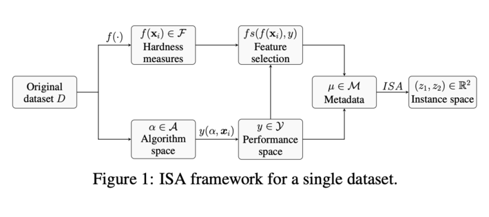
Picture taken from paper
Where,
- D: Dataset
- xi: ith observation
- F: Set of hardness measures
- A: Set of algorithms. Bagging, Gradient Boosting, Support Vector Machine (both linear and RBF kernels), Logistic Regression, Multilayer Perceptron, Random Forest, dummy and gaussian naïve bayes
- Y: Value of performance metrics of each algorithm on each instance
- M: Joined dataset of F and Y
Some Definitions:
Lets look at some of the definitions we need to know in order to understand the overall algorithm. I will try to make it as simple as possible. For more technical detail, please refer to the original paper.
Hardness Measures:
First lets introduce Instance Hardness, which basically tells, how hard it is to classify an instance by algorithms. The formal definition of the same is as below:
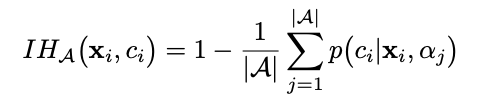 Where,
|A| : No. of algorithms used
p(ci|xi,aj) : Probability of instance xi being classified as ci by model aj
In simple terms, Instance Hardness of an instance xi for class ci, is the average likelihood of an instance to be misclassified for class ci by the algorithm set. Higher the IH, harder the instance to be correctly classified for class ci. We will majorly look at IH to understand the instances hardness to classify.
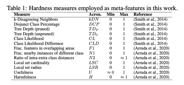
There are other hardness measures which have been used to create the meta-features of the dataset. These are majorly fed into the ISA model to create the 2D hardness embedding. They are as below:
Algorithm performance:
Each algorithms performance on each instance is done using cross validation. As per the source code, average cross-validation score, with 10 folds, is estimated over 10 iterations for each instance. The cross-validation strategy is made in a way, such that each instance belongs to at least one test set.
Feature Selection:
A supervised feature selection is done on the meta-feature set (set of hardness measures) to keep only the most informative features. We will not go into the detail of the same in this article.
IS representation and footprint:
Instance Space (IS) representation is done using the Python package named PyIspace which is the package which implements Instance Space Analysis. Additionally, a rotation adjustment is done so that the hard-to-classify instances is plotted on the top left corner of the graph. Also, footprint areas (area for easy-to-classify instances) are defined consisting of instances with IH < 0.4
Algorithm step by step:
Below are the steps which are followed by default:
- Run hardness measures on all the observations to create the meta-features
- Select most informative meta-features
- Run all algorithms on all observations to get average log-loss error across cross validation sets
- Concatenate 2 and 3 to get the meta-dataset
- Calculate Instance Hardness values
- Run ISA model on the metadata (got in 4) to get rotation adjusted 2D coordinates of the instances and footprints
- Plot instances along with the footprints for visual inspection of the Instance Hardness
Example and code:
The package can be found in the link:
https://gitlab.com/ita-ml/pyhard/-/tree/master
However, for the demonstration here, I will consider the data used in the paper, look at some specific code snippet which can be run separately and get the desired results. Below are the points, from the above link, regarding the input data:
- Only csv files are accepted
- Do not include any index column. Instances will be indexed in order, starting from 1
- The last column must contain the classes of the instances
- Categorical features should be handled previously
The dataset contains anonymized data from citizens (total 5156 citizens) positively diagnosed for COVID-19, collected from March 1st, 2020 to April 15th, 2021. It involves predictions of whether an individual will require future hospitalization taking various symptoms and comorbidities as input. The data (df) looks like below:
Table 2: Top rows of the raw data

Our objective is to identify the citizens who are difficult to classify by most of the models. As well as the citizens who are easy to classify.
First, calculate the hardness measures and store it in a dataframe:
import pandas as pd
from pyhard.measures import ClassificationMeasures
m = ClassificationMeasures(df)
df_meta_feat = m.calculate_all()
Keep scores (average log-loss error) of all the algorithms for all instances in a dataframe:
from pyhard.classification import Classifier
clf = Classifier(df)
df_algo = clf.run_all()
Create metadata:
df_metadata = pd.concat([df_meta_feat, df_algo], axis=1)
Calculate IH values for all the instances and store it in a dataframe:
ih_values = clf.estimate_ih()
n_inst = len(df_metadata)
df_ih = pd.DataFrame({‘instance_hardness’: ih_values},index=pd.Index(range(1, n_inst + 1), name=instances_index))
Next, run the ISA model to get the 2D representation on the metadata:
from pyhard import integrator
from pathlib import Path
from pyispace.trace import trace_build_wrapper, make_summary, _empty_footprint
from pyispace.pilot import PilotOutput, pilot, adjust_rotation
n_classes = df.iloc[:, -1].nunique()
epsilon = loss_threshold(n_classes, metric=’logloss’) #Calculates the maximum threshold below which the metric indicates a correct classification of the instance
other = {‘perf’: {‘epsilon’: epsilon}}
model = integrator.run_isa(rootdir=Path(.), metadata=df_metadata, settings=other,
rotation_adjust= True, save_output=False)
threshold = 0.4
pi = 0.55
Ybin = df_ih.values[:, 0] <= threshold
ih_fp = trace_build_wrapper(model.pilot.Z, Ybin, pi)
The result can be saved in the root_dir path by running the below:
from pyispace.utils import save_footprint, scriptcsv
save_footprint(ih_fp, rootdir_path, ‘instance_hardness’)
scriptcsv(model, rootdir_path)
Among the files saved, there will be two files named coordinates.csv and footprint_instance_hardness_good.csv. The first one gives the coordinates for each instance. These are the 2D embedding of the metadata (z_1 and z_2 in the below graph). The second one gives the footprint co-ordinates as per Instance Hardness. These can be plotted for the visual inspection. Authors have also built a beautiful and interactive visualization App which can also be hosted in local system very easily. Below is a screenshot of the same:
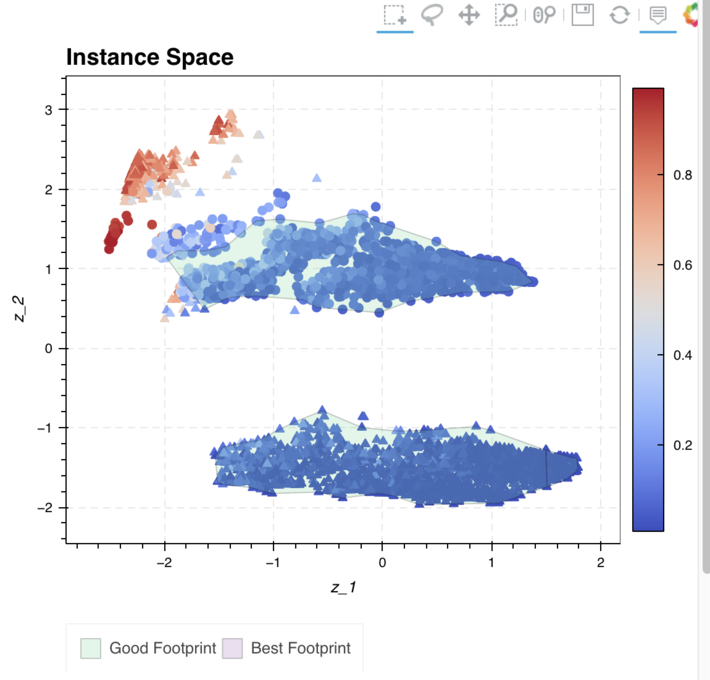 Figure 2: Screenshot of a part of the visualization App
Conclusion:
PyHard is a great package that can be used in many ways to explore a dataset and the observations. It can easily identify noisy and anomalous observations within a dataset and at the same time, it can also help in determining different model performance on the instances. It also provides a beautiful visualization tool which helps in identifying easy as well as hard instances to classify in 2D space.