
PREFACE
Previously, I tackled the Gambler’s Ruin problem using conditional probability and difference equations as well as visualising the simulations of the problem in a random walk style using Python/Pygame. This can be found here: https://www.datasciencecentral.com/profiles/blogs/gambler-s-ruin-si….
Continuing this gambling style, the following demonstrates a simple application of Bayesian Inference, probability generating functions and conjugacy to a process involving multiple random variables.
This article has 5 sections:
0- Introduction: Introduction to a process dependent on two random variables
1- The Problem: Setting up the wheel of fortune problem
2- The Solution: The solution to the wheel of fortune problem
3- Finding the probability p from observations: Theory for applying Bayesian Inference to the problem
4- Simulations: Simulations of the problem and the application of the theory to infer a posterior probability distribution for a parameter
The full code (Jupyter Notebook) and theory can be found here: https://github.com/TanselArif-21/WheelofFortune
INTRODUCTION
It is sometimes the case that a random variable is dependent upon another random variable. For example, on some slot machines, the number of spins of the bonus wheel depends on the number of spin/bonus icons you achieve on the slots wheel itself. If you get 1 spin icon you get to spin the wheel once, if you get 2 spin icons, you get to spin the wheel twice and so on. If there is a certain probability of winning the bonus in the wheel each time you spin it and the wins from each spin are independent, then the more times you’re allowed to spin it, the more chance of winning the bonus. But, the number of initial spin icons determines the number of times you’re allowed to spin the wheel which in turn give you more chances to win the bonus. The question is, what is the probability of winning the bonus each time you play?
Additionally, suppose the probability distribution of the slots is known but not that of the wheel. Given observations on the history of the games played and the results of those games, it is possible to make some guess on the probability distribution of the wheel that would most likely result in such data. We will approach this part of the problem by thinking in a Bayesian context.
Below, I frame a similar problem with a wheel and coin flips to simplify the work a little.
THE PROBLEM
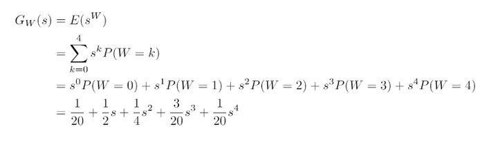
You spin the wheel of fortune. The wheel gives 0 with probability 1/20, 1 with probability 1/2, 2 with probability 1/4, 3 with probability 3/20 and 4 with probability 1/20.
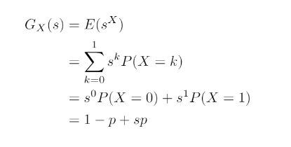
Depending on the number you get from the wheel, you are allowed to flip a coin that many times and record the number of heads you get. The coin is biased towards heads with a probability of 7/10 of getting a heads.
What is the probability distribution of the number of heads if you play the game?
THE SOLUTION
We note that a random variable (Y) representing the number of heads per game depends on the random variable (W) representing the number from a spin of the wheel and the random variable (X) representing a flip of the coin. We can use the probability generating function of W and X to find the probability generating function of Y and subsequently the probability distribution of Y. Hence solving the problem of a case of dependent processes. This gives us a starting point to think about applying Bayesian Inference to the case where one of these processes have unknown distributions.
In particular, the probability generating function for W (representing the value obtained from the wheel) is:
And the probability generating function for X is:
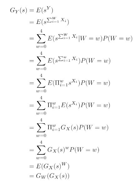
Allowing the derivation of the probability generating function for Y using:
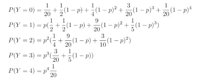
Resulting in the following probability distribution for Y – the total number of heads:
FINDING THE PROBABILITY p FROM OBSERVATIONS
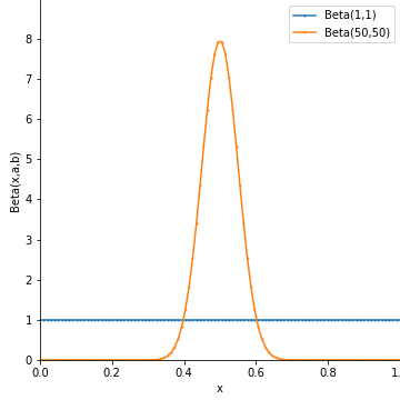
Suppose that we are not told the value of p (probability of heads in a coin flip). Given an observation of W, Y has a more well-known distribution. In particular, Y depends on a fixed number of coin flips. Y then has a Binomial Distribution. If we choose a Beta(1,1) prior distribution for p, this enables the simplification of the problem since the Beta Distribution is a conjugate prior of the Binomial Distribution.
A plot of Beta(1,1) (uniform distribution) and Beta(50,50) can be seen in the image below:
Applying a Beta(1,1) prior distribution to p, and noting that the data (Y) comes from a Binomial distribution, the posterior distribution for p has the distribution:
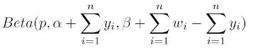
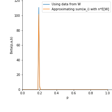
where the parameters of the distribution have been updated using the observed values for Y and W. Note that even if the data for the outcomes from W is not accessible to us, we can still estimate the sum above using the expected value for W as N E[W]. This posterior distribution using values from the simulation (code given in the next section) can be seen in the image below to accurately estimate p as 0.2 (the orange line estimates the parameter in the Beta distribution without seeing data from W whereas the blue line uses actual observed data):
SIMULATIONS
Below, we can see a simulation of 10000 runs through the problem:
# Import modules
from scipy import stats
import math
import numpy
# Set the seed
np.random.seed(101)
# Build W by concatenation of lists
w = []
w.append(0)
w.extend([1]*10+[2]*5+[3]*3+[4]*1)
# Set the probability of heads from a coin flip
p = 0.2
# Set the number of games
n = 10000
# Initialise the total number of heads obtained
y_outcome = 0
# Get n samples from w
w_outcome = np.random.choice(w,size=n)
# For each w, flip the coin that many times
y_outcome = [np.sum(stats.bernoulli.rvs(p,size=this_w)) for this_w in w_outcome]
y_sum = sum(y_outcome)
w_sum = sum(w_outcome)
print(‘Total number of heads = {}’.format(y_sum))
print(‘Total number of coin flips = {}’.format(w_sum))
Below we can utilise the theory in the previous section to derive the probability p from the data using the Beta distribution:
# Get figure object
fig = plt.figure(figsize=(5, 5))
# Get axes object
axes = fig.add_axes([0.2,0.2,0.8,0.8])
# Create a numpy array of 100 points equally spaced
x = np.linspace(0,1,100)
# Create a numpy array of the posterior distribution using actual observed values of W
y = np.array([stats.beta.pdf(i,1+y_sum,1-y_sum+w_sum) for i in x])
# Create a numpy array of the posterior distribution by estimating sum(W) with it’s expected value
z = np.array([stats.beta.pdf(i,1+y_sum,1-y_sum+n*1.65) for i in x])
# Plot onto the axes
axes.plot(x, y, ‘-o’,ms=0,label=’Using data from W’)
axes.plot(x, z, ‘-o’,ms=0,label=’Approximating sum(w_i) with n*E[W]’)
# Set the axis labels
axes.set_xlabel(‘p’)
axes.set_ylabel(‘Beta(p,a,b)’)
# Show legend
axes.legend()
# Set axis limits
axes.set_xlim(0,1.05)
axes.set_ylim(0,max(y.max(),z.max())+10)
# Remove some borders
axes.spines[‘right’].set_visible(False)
axes.spines[‘top’].set_visible(False)
Read in full here: https://github.com/TanselArif-21/WheelofFortune