
PREFACE
This article has 4 sections:
- Introduction: Introduction to the gambler’s ruin problem
- Methodology: How the simulation will be carried out
- Pseudocode: Summary of the Python Code
- Theory: A summary of the theory
The full code and theory can be found here: https://github.com/TanselArif-21/GamblersRuin
INTRODUCTION
The Gambler’s Ruin problem frames a gambler who begins gambling with an initial fortune – in dollars say. At each successive gamble, the gambler either loses $1 or gains $1. This means that the gambler’s fortune after this gamble is only dependent on their current fortune and not how the fortune ended up at this value. The problem is to find the probability that the gambler goes bankrupt – loses the entirety of the fortune. This problem is a kind of random walk.
I will use Pygame to visualise the trajectories and the simulation in the order they are conducted. The Video below shows this simulation in action at normal speed. Every time a trajectory hits the red line (bankruptcy line), the number of bankruptcies as well as the number of simulations increases by 1. Every time a trajectory hits the upper green line (the take profit line), only the number of simulations is increased by 1 but not the number of bankruptcies. Each simulation trajectory is represented by a random colour (RGB value):
Below is a faster simulation consisting of 500 individual simulations:
And here’s an image of the results for 1000 simulations:
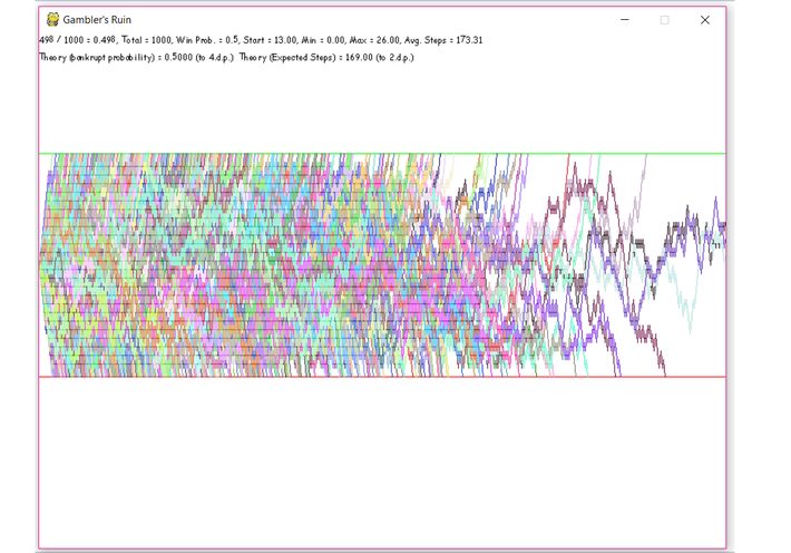
The more the simulations, the better the approximation of the theoretical value.
Methodology
We will begin with an initial fortune $F. We will then sample from a Bernoulli random variable with probability of success p. If this distribution produces a success, the fortune at the next step will be $(F+1). If this distribution produces a fail, the fortune at the next step will be $(F-1).
This process is repeated until either: a- The fortune reaches $0, or b- The fortune reaches some specified value $N, at which point the process stops
We will call the entire procedure above, a single simulation of the gambler’s fortune. After carrying out many of these simulations, we can obtain an estimate of the bankruptcy probability by taking all the simulations where the fortune reached $0, and divide this by the total number of simulations.
Additionally, we can count the number of steps per simulation and calculate the mean number of steps before the gambler either goes bankrupt or takes their profit and walks away.
For the visualisation of this process, we will use Pygame. Pygame has a pygame.draw.line function which allows a simple line to be drawn on the canvas by specifying the line’s starting point, ending point and its colour. So, at each step of a single simulation, if we define a line with its starting point as the current fortune and the ending point the fortune at the next step, we will have defined a line to be drawn by the previously mentioned function. A list of line objects can be formed in this way and then drawn on the canvas one by one to form a visual representation of a simulation.
The next section will give more insight into the pseudocode of this app.
PSEUDOCODE
Import the following libraries:
import pygame # For the visualisation
import random # For the generation of random numbers so that each simulation has a random colour
from scipy import stats # For simple sampling from a Bernoulli random variable
Create a class called ‘Line’ containing a start value, an end value and a colour:
class Line:
# Some code
Define a function to deal with drawing a list of lines to the canvas:
def draw_canvas(lines, count, step, theory):
”’
A function tasked with drawing lines to the screen.
:param lines: a list of line objects to draw
:param count: a list of 0’s and 1’s where a 1 means bankruptcy at that step
:param step: an integer to specify which step in the simulation to display to
:param theory: a list of 2 floats containing [theoretical probability, theoretical expected steps]
”’
# Some code containing the following code: pygame.draw.line(game_display, line.color, line.start, line.end)
Define a function to deal with the stop condition:
def stop(y, min_y, max_y):
”’
A function which checks the stop conditions.
:param y: current value
:param min_y: upper limit in screen terms
:param max_y: lower limit in screen terms
:return: -1 = do not stop, 0 = stop due to bankruptcy, 1 = stop due to becoming rich
”’
# Some code
Define a function to deal with a single sample from the Bernoulli distribution:
def get_next_value(p):
”’
A function which returns a 1 or a -1. p is the probability of obtaining a 1
:param p: float between 0 and 1. The probability of success
:return: integer. Either -1 or 1
”’
# Some code
Define a function to deal with the propagation of a single trajectory/simulation:
def propagate(start, minimum, maximum):
”’
A function which simulates the trajectories for the current fortune. This function returns 2 data structures: A list containing the the trajectory value concatenated, and a list of the same size containing information on whether that step resulted in a bankruptcy or not
:param start: float between minimum and maximum. Starting amount
:param minimum: float. Amount defining bankruptcy
:param maximum: float. Amount above which take win is actioned
:return: list, list
”’
# Some code
Define a main function to run the propagation of multiple simulations:
def main():
# Some code
The full annotated code can be found here.
THEORY
The theoretical solution to the probability of bankruptcy involves forming a difference equation by conditioning the probability of bankruptcy on the first gamble:
u_k = P(wins first gamble) × u_{k+1} + P(loses first gamble) × u_{k−1}
The theoretical solution to the expected number of steps is also conditioned on the first gamble:
n=p×(1+E_{n+1}) +q×(1+E_{n−1})
where u_i and E_i are the probability of bankruptcy and expected number of steps with initial fortune i respectively.
The full theory and derivation can be found here.