Scale-Invariant Clustering and Regression

The impact of a change of scale, for instance using years instead of days as the unit of measurement for one variable in a clustering problem, can be dramatic. It can result in a totally different cluster structure. Frequently, this is not a desirable property, yet it is rarely mentioned in textbooks. I think all clustering software should state in their user guide, that the algorithm is sensitive to scale.

We illustrate the problem here, and propose a scale-invariant methodology for clustering. It applies to all clustering algorithms, as it consists of normalizing the observations before classifying the data points. It is not a magic solution, and it has its own drawbacks as we will see. In the case of linear regression, there is indeed no problem, and this is one of the few strengths of this technique.

Scale-invariant clustering

The problem may not be noticeable at first glance, especially in Excel, as charts are by default always re-scaled in spreadsheets (or when using charts in R or Python, for that matter). For simplicity, we consider here two clusters, see figure below.

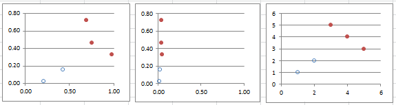
Original data (left), X-axis re-scaled (middle), scale-invariant clustering (right)

The middle chart is obtained after re-scaling the X-axis, and as a result, the two-clusters structure is lost. Or maybe it is the one on the left-hand side that is wrong. Or both. Astute journalists and even researchers actually exploit this issue to present misleading, usually politically motivated, analyses. Students working on a clustering problem might not even be aware of the issue.

On the right-hand chart, we replaced each value for each axis, by their rank in the data set: it solves the problem, as re-scaling (or even applying any monotonic, non-linear transformation) preserves the order statistics (the ranks). Another way to do it is by normalizing each variable, so that the variance for each variable, after normalization, is equal to 1. Using the ranks is a better, more robust, noise-insensitive approach though, especially if the variables have a relatively uni-modal distribution (with no big gaps), as in the above figure.

The main issue with scale-invariant clustering appears in the context of supervised classification. When adding new points to the training set, the augmented training set needs to be re-scaled again. There is no distance or similarity metric (the core metric used in clustering algorithms, be it K-NN, centroid or hierarchical clustering) that will consistently preserve the initial clustering structure after adding new points and re-scaling. See exercise in the last section for a (failed) attempt to build such a distance. However, see my article on scale-invariant variance, which leads to a very weird kind of “variance” concept.

Scale-invariant regression

By design, linear regression is, in some way, scale-invariant. The fact is intuitive and certainly very easy to prove, and it is illustrated in our spreadsheet (see next section.) In short, if you multiply one or more dependent variable by a factor (which amounts to re-scaling them) then the corresponding regression coefficients will be inversely re-scaled by the same factor. To put it differently, if one dependent variable is measured in kilometers, and its attached regression coefficient is (say) 3.7, then if you change the measurement from kilometers to meters, its regression coefficient will change from 3.7 to 3.7 / 1000. This makes perfect sense, yet I don’t remember having learned this fact in college classes nor textbooks.

Note that this works only if the re-scaling is linear. If you use a logarithm transformation instead, then this property is lost. Some authors have developed rank-regression techniques to handle non-linear re-scaling, using the same approach as in the previous section on clustering.

Excel spreadsheet with computations

To download the spreadsheet with the computations, click here. Probably the most interesting feature of the spreadsheet is to help you learn how to do linear regression in Excel, and how to produce scatter-plots with multiple clusters as in the above figure.

It is interesting to note that the 5 points in the above figure were all generated using random deviates on [0, 1] with the Excel function RAND(). Despite being “random”, these points seem to exhibit a structure made of two clusters. This is a typical result: random points always exhibit some patterns (in particular, weak clustering, holes, weak linear structures and twin points.) See for instance this article. It is possible to test if these structures found in any data set are weak enough, yet not too weak, given the size of the data set, to assess whether it is a result of natural patterns found in randomness, or not. The easiest way to test this is by using Monte-Carlo simulations. If the points were too evenly distributed, they would not be the result of a random distribution.

So in the above figure, the two apparent clusters are an artifact or an optical illusion, and can not be explained by any causal model. Repeat this experiment a thousand times, and you will find similar clusters in a majority of your simulations.

Exercise

Let’s try to create a scale-invariant distance d between two points x = (x1, x2) and y = (y1, y2) using this formula:

Prove the following:

and is thus not scale-invariant. It is proportional to the infinity norm distance. How does it generalize to more than two variables? Note that the the supremum in the first formula is attained either with (a, b) = (1, 0) or (a, b) = (0, 1). The case (a, b) = (1, 1) corresponds to the classic Euclidean distance.

For related articles from the same author, click here or visit www.VincentGranville.com. Follow me on on LinkedIn.

DSC Resources