

Limitations on physical interactions throughout the world have reshaped our lives and habits. And while the pandemic has been disrupting the majority of industries, e-commerce has been thriving. This article covers how reinforcement learning for dynamic pricing helps retailers refine their pricing strategies to increase profitability and boost customer engagement and loyalty.
In dynamic pricing, we want an agent to set optimal prices based on market conditions. In terms of RL concepts, actions are all of the possible prices and states, market conditions, except for the current price of the product or service.
Usually, it is incredibly problematic to train an agent from an interaction with a real-world market. The reason is that an agent should gain lots of samples from an environment, which is a very time-consuming process. Also, there exists an exploration-exploitation trade-off. It means that an agent should visit a representable subset of the whole state space, trying out different actions. Consequently, an agent will act sub-optimally while training and could lose lots of money for a company.
An alternative approach is to use a simulation of the environment. Using a prognostication model, we can compute the reward (for example, income) based on the state (market conditions, except current price), and the action is the current price. So, we only need to model transitions between states. This task strongly depends on the state representation, but it tends to create a few modelling assumptions to be solved. The main drawback of the RL approach is that it is extremely hard to simulate a market accurately.
Sales data
For simplicity, we use simulated sales rather than real ones. Sales data are simulated as a sum of a price-dependent component, a highly seasonal component dependent on time and a noise term. To get a seasonal component, we use the Google Trends data of a highly seasonal product a swimming pool. Google Trends provides weekly data for over five years. There is a clear one-year seasonality in the data, so it is easy to extract it and use it as a first additive term for sales. Since this term repeats with the one year, it is a function of a week number, ranging from 0 to 52.

The second term depends on prices from the current timestamp as well as the previous timestamp to model sales. The overall formula looks like this:

Here, f may be any monotonically decreasing function. The intuition is that if all other features are fixed, increasing the companys price (either current or previous) decreases sales. On the other hand, increasing competitors prices leads to increased sales. The random term is sampled from a zero-mean normal distribution.

We set the function f to be linear with a negative coefficient. This allows us to analytically find a greedy policy and compare it with the RL agents performance.
Experiments
We treat the dynamic pricing task as an episodic task with a one-year duration, consisting of 52 consecutive steps. We assume that competitors change their prices randomly.
We compare different agents by running 500 simulations and collecting cumulative rewards over 52 weeks. The graph below shows the performance of the random and greedy agents

Tabular Q-learning
Q-learning is an off-policy temporal difference control algorithm. Its main purpose is to iteratively find the action values of an optimal policy (optimal action values).

Using these action values, we can easily find an optimal policy. It would be any greedy policy with respect to optimal action values. The following updated formula is used:

The estimates converge to the optimal action values, independent of the policy used (usually epsilon-greedy with respect to the current estimates is used). This updated formula can also be treated as an iterative way of solving Bellman optimality equations.
This algorithm assumes a discrete state space and action space. Accordingly, before running this algorithm, we should discretise continuous variables into bins. The name tabular means that action values are stored in one huge table. Memory usage and training time grow exponentially with the increase in the number of features in the state representation, making it computationally intractable for complex environments (for example Atari games).


As we can see, this approach outperforms a random agent, but cannot outperform a greedy agent.
Deep Q-network
The deep Q-network (DQN) algorithm is based on the same idea as Tabular Q-learning. The main difference is that DQN uses a parametrised function to approximate optimal action values. More specifically, DQN uses artificial neural networks (ANNs) as approximators. Based on state representation, both convolutional neural networks and recurrent neural networks can be used.

The optimisation objective at iteration i looks as follows:

where:

The behaviour distribution p is obtained by acting epsilon-greedy with respect to the previous models parameters.
The gradient of the objective is as follows:

The loss function is optimised by stochastic gradient descent. Instead of computing a full expectation, a single-sample approximation can be used, leading to an updated Q-learning formula.
Two problems that make the optimisation process harder are correlated input data and the dependence of the target on the models parameters. Both problems are tackled by using an experience replay mechanism. At each step it saves a trajectory into a buffer, then instead of using a single trajectory to update parameters, a full batch sampled from a buffer is used.
With DQN you can use higher-dimensional state spaces (even images can be used). Also, it tends to be more sample-efficient than the Tabular approach. The reason is that ANNs can generalise to unseen states, even if the agent does not act from those states. On the other hand, the Tabular approach requires the whole state space to be visited. DQN is sample-efficient because it is an experience replay, which allows multiple uses of a single sample.


As we can see, DQN outperforms all other agents. Also, it was trained on a smaller number of episodes.
Policy Gradients
The policy gradients algorithm uses an entirely different idea to learn an optimal policy. Instead of learning optimal action values and moving greedily with respect to them, policy gradients directly parametrise and optimise a policy. ANNs are often used to parametrise a policy.

The difficulty here is that an optimisation objective, the state-value of the first state, depends on a dynamics function p, which is unknown.

That is why policy gradients use the fact that the gradient of the objective is an expected value of a random variable, which is approximated while acting in the environment.

We can subtract a baseline, which depends only on the state, from action value estimates to reduce variance. This does not affect the mean but can significantly reduce the variance, thus speeding up the learning process.

Usually, state-value estimates are used as a baseline.
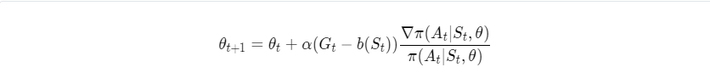
Then stochastic gradient ascent is done using the following formula:
This method requires a lot of interaction with an environment in order to converge.


Policy gradients outperform a greedy agent but do not perform as well as DQN. Likewise, policy gradients require far more episodes then DQN.
Please note that the real-world market environment and dependencies in it are way more complicated. This article covers a basic simulation proving that approach is working and can be applied to real data.
We will be happy to answer your questions. Get in touch with us any time!
Originally published at ELEKS Labs blog.