
Bayesian inference is the re-allocation of credibilities over possibilities [Krutschke 2015]. This means that a bayesian statistician has an “a priori” opinion regarding the probabilities of an event:
p(d) (1)
By observing new data x, the statistician will adjust his opinions to get the “a posteriori” probabilities.
p(d|x) (2)
The conditional probability of an event d given x is the share of the joint probability (d and x) of x.
p(d|x) = p(x,d) / p(x) –> p(d|x) p(x) = p(x, d) (3)
reverse:
p(x|d) = p(x,d) / p(d) –> p(x|d) p(d) = p(x, d) (4)
setting (4) in (3):
p(d|x) = p(x|d) p(d) / p(x) (5)
Which is the Bayes theorem.
p(x) represents the sum of all joint probabilities p(x,dj) for each event j of d. In this regard, d can either be dichotomous [1,0], a set of categories [1, 2, …, n], [computing the probability of category j of d:]
p(dj|x) = p(x|dj) p(d) / j=1 to n∑p(x|dj) p(dj) (6)
or the denominator can be assumed with infinite categories. This is used to obtain information about all possible states between the categories. For example, if d is dichotomous [0, 1] and the probability of d = 0.2 is desired. In this case, the sum over d gets an integral, which is not solvable.
p(dj|x) = p(x|dj) p(dj) / ∫p(x|d) p(d) dd (7)
Note that one can approximate the integral for example with conjugate distributions or with Marcov Chain Monte Carlo simulations.
Merely for classification, this case (7) is not necessarily relevant. Except one would like to predict the whole a posteriori distribution.
What if we want to use more than one variable for prediction?
Normally, the joint probability of e.g. d, x, and y is calculated with the chain rule for probabilities:
p(d, x, y) = p(d|x,y)∙p(x|y)∙p(y) (8)
For simplification, in the case of two or more variables the Naive Bayes Classifier [NBC] assumes conditional independence. Even in the case of a violation of the independence assumption the classifier performs well [see. Domingos, Pazzani, 1997]. Looking at the last two factors of equation (8). Supposed x would be independent from y. In this case is
p(x|y) = p(x) (9)
because y does not affect x. Inserted in the Bayes theorem equation:
p(x) = p(y, x) / p(y) –> p(x)∙p(y) = p(x, y) (10)
So, one can proof whether there is conditional independence or not.
For the NBC, in case of two variables x and y the conditional independence assumption leads to:
p(d|x,y) = p(x,y|d) p(d) / p(x,y) (11)
= p(x|d) p(y|d) p(d) / p(x|d) p(y|d) p(d) + p(x|⌐d) p(y|⌐d) p(⌐d) (12)
Thus, using k variables:
p(dj|x) = p(dj) ∙ i=1 to k∏p(xi|dj) / j=1 to n∑ p(dj) ∙ i=1 to k∏p(xi|dj) (13)
- A certain class dj given the vector x is the a priori probability p(dj) times
- the likelihood i=1 to k∏p(xi|dj) on the assumption of independent variables divided through
- the evidence j=1 to n∑ p(dj)∙i=1 to k∏p(xi|dj) which is equal to the joint probability p(x1, x2, x3, …, xk).
How to calculate the individual probabilities?
For each dj, the probability p(dj) is just #dj / #observations.
For example, if there are 100 observations with a = 20, b = 30, and c = 50, p(da) is 20%.
In contrast, the likelihoods are conditional. They refer just to the number of observations which are labeled with dj. If x is categorical e.g. [I, II, III] the likelihood p(x = II|da) is #observations where x = II divided through # da. For example xI = 2, xII = 8, xIII = 10, p(x = II|da) is 8/20 = 40%.
Frequently, there are continuous variables in practice. For continuous variables one needs the probability of a realization of x within all observations of x. To determine these probabilities a density function is proposed. To get suitable results it is important to ensure an appropriate approximation. With a soaring number of attributes, it is time consuming to look at all distributions at hand. In the best case the features result directly from a feature engineering which gives a hint, which kind of distribution occurs. For example, a feature is engineered which consists of standard deviations from other features. In such a case, the distribution might be Chi square. One further approach is to assume normal distribution. In this case the standard deviation and the mean must be computed. Another approach is to built categories and measure how often a particular observation falls into a certain category – which works well.
The problem is that a wrong assumption can bias the result. Distributions can take diverse shapes. For example, the observations can be concentrated at different positions (multimodal or leptokurtic). Or, there could be skewness. The specification of a shape in advance can bias the prediction of the a posteriori – if the truth is too far removed from reality.
So, the idea is to determine the shape by a Kernel Density Estimation [KDE] like proposed by John and Langley 1995.
Kernel Density Estimation
A KDE weights a defined density around each observation xr equally first. In this regard, a kernel function K is needed – e.g. a normal, triangular, epanechnikov or uniform distribution. The next step is to sum up all densities to get a density function.
KDE(x) = 1/hm ∙ r=1 to m∑K((x-xr) / h) (14)
Assumed we would use a normal distribution. The xr can be interpreted as mean where the distribution is centered around. The h can be interpreted as standard deviation, so it is called bandwidth. Each distribution K((x-xr) / h) of the m observations is weighted equally with 1/m.
One can proof that the integral of KDE(x) equals one by looking at the contribution of each term.
∫1/hm ∙ K((x-xr) / h) dx (15)
((x-xr) / h) = y (16)
dx = h∙dy (17)
we know that ∫K((x-xr) / h) = 1, so:
1/m ∫K(y) dy = 1/m (18)
The sum of the integrals is 1/m ∙ m = 1.
An important factor is the bandwidth h. The higher the h the smoother the distribution.
The following figure shows a variety of h = [0.1, 0.5, 1].
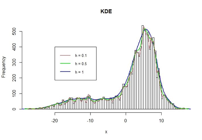
Note: For adjustment, the KDEs are multiplied with a factor (max frequency/max Density)
Setting h too small can end up in high variance whereas setting h too high can lead to bias.
So, lets go through an fictional example in R.
#d is dichotomous and created as 30% of 10.000 observations d = 1.
d = rep(0, times = 7000)
d = c(d, rep(1, times = 3000))
#m and s are mean and standard deviation for the random normal distribution. mi and ma are min
#and max for random uniform distribution.
m = 5; s = 3; mi = 0.1; ma = 5
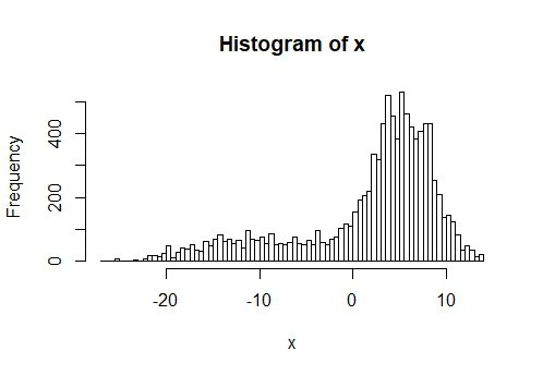
#Creating highly correlated features x and y.
set.seed(123)
x = runif(1000, min = mi, max = ma) * 0.2 + rnorm(1000, mean = m, sd = s) +
d * -10 * runif(1000, min = mi / 2, max = ma / 2)
hist(x, nclass = 100)
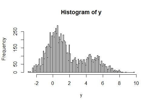
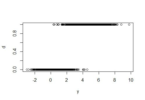
y = -0.1*x+rnorm(1000, mean = 1, sd = 1.16)+3*d
hist(y, nclass = 100)
#Correlation between x and y is about -78%
cor(x, y); cor(y, d)
plot(x, d)
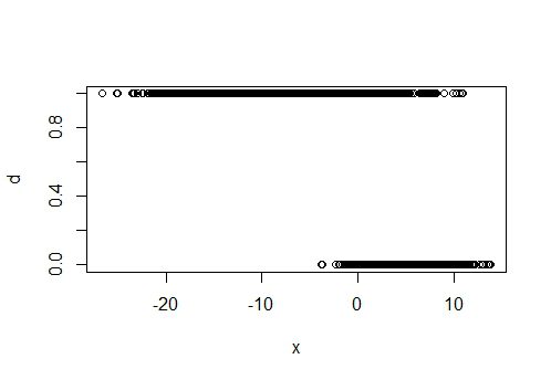
plot(y, d)
###TEST DATA####
dt = rep(0, times = 7000)
dt = c(dt, rep(1, times = 3000))
#change the distribution parameters to take occurring trends into account
mt = 5.1; st = 2.9; mit = 0.2; mat = 4.9
set.seed(321)
xt = runif(1000, min = mit, max = mat) * 0.2 + rnorm(1000, mean = mt, sd = st) +
dt * -10 * runif(1000, min = mit / 2, max = mat / 2)
hist(xt, nclass = 100)
yt = -0.1*xt+rnorm(1000, mean = 1, sd = 1.16)+3*dt
hist(yt, nclass = 100)
cor(xt, yt); cor(yt, dt)
plot(xt,d); plot(yt,d)
#Computing the prior probabilities. Actually, they does not have to be calculated for this example 😉
a_priori = sum(d)/length(d)
a_PrioriNOT = 1 – sum(d)/length(d)
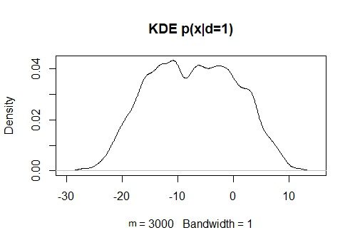
#Computing the KDE for x and y given d = 1 and d = 0. This ist the model training.
KDxd1 = density(x[d==1], bw = 1)
plot(KDxd1, main = “KDE p(x|d=1)”)
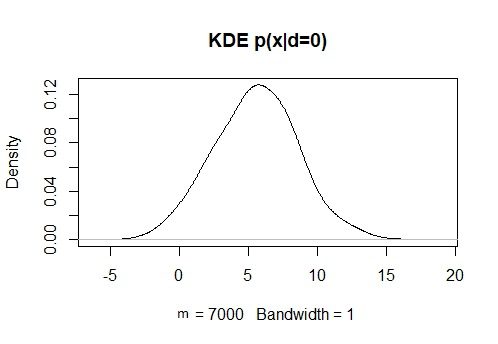
 KDxd0 = density(x[d==0], bw = 1)
plot(KDxd0, main = “KDE p(x|d=0)”)
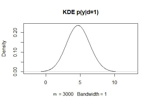
KDy1 = density(y[d==1], bw = 1)
plot(KDy1, main = “KDE p(y|d=1)”)
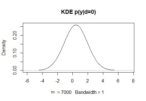
KDy0 = density(y[d==0], bw = 1)
plot(KDy0, main = “KDE p(y|d=0)”)
#Computing the likelihoods p(x|d=1), p(x|d=0), p(y|d=1), and p(y|d=0). The approx function
#calculates a linear approximation between given points of the KDE:
likelyhoodx1 = approx(x = KDxd1$x, KDxd1$y, xt, yleft = 0.00001, yright = 0.00001)
likelyhoodx0 = approx(x = KDxd0$x, KDxd0$y, xt, yleft = 0.00001, yright = 0.00001)
likelyhoody1 = approx(x = KDy1$x, KDy1$y, yt, yleft = 0.00001, yright = 0.00001)
likelyhoody0 = approx(x = KDy0$x, KDy0$y, yt, yleft = 0.00001, yright = 0.00001)
#Computing the evidence. Note: the likelihoodxxx$y is the density:
evidence = likelyhoody1$y*likelyhoodx1$y*a_priori+likelyhoody0$y*likelyhoodx0$y*a_PrioriNOT
#Computing the a posteriori probability by using Bayes theorem:
a_posteriori = likelyhoody1$y*likelyhoodx1$y*a_priori/evidence
#assigning the prediction with a cutoff of 50%.
prediction = ifelse(a_posteriori > 0.5, 1, 0)
#calculating content of confusion matrix
hit1 = ifelse(prediction == 1 & dt == 1, 1, 0)
false1 = ifelse(prediction == 1 & dt == 0, 1, 0)
hit0 = ifelse(prediction == 0 & dt == 0, 1, 0)
false0 = ifelse(prediction == 0 & dt == 1, 1, 0)
#Creating confusion matrix
Confusion <- matrix(c(sum(hit1), sum(false0), sum(false1), sum(hit0)), nrow = 2, ncol = 2)
colnames(Confusion) <- c(“d = 1”, “d = 0”)
rownames(Confusion) <- c(“p(d = 1|x,y)”, “p(d = 0|x,y)”)
| Confusion | d = 1 | d = 0 |
| p(d = 1|x,y) | 2718 | 56 |
| p(d = 0|x,y) | 282 | 6944 |
Note that this is an example to show hot you can apply NBC with KDE. the example is constructed and not represenative regarding the power of KDE.
#Looking at the areas where misclassifications occur. Red = misclassification; Black = correct classified:
color = ifelse(prediction == dt, 1, 2)
plot(xt, dt, col = color)
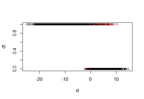
plot(yt, dt, col = color)
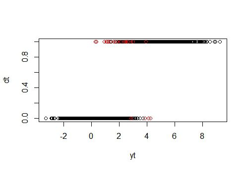
As expected, most misclassifications are in the overlapping areas in the minority class. But the combination of both x any y more often leads to correct classifications – even in the overlapping areas. Considering that there is a high correlation between x and y, this result shows that even in case of violating the conditional independence assumption, the NBC performs well.
Sources:
Domingos, P & Pazzani, M. (1997). On the Optimality of the Simple Bayesian Classifier under Zero-One Loss. Machine Learning, 29, (pp. 103–130)
John, G., & Langley, P. (1995). Estimating continuous distributions in Bayesian classifiers. Proceedings of the Eleventh Conference on Uncertainty in Artificial Intelligence (pp. 338–345). Montreal, Canada: Morgan Kaufmann.
Krutschke, J (2015). Doing Bayesian Data Analysis. A Tutorial with R, JAGS, and Stan. Second Edition. Academic Press of Elsevir.
)