Sales data analyses can provide a wealth of insights for any business but rarely is it made available to the public. In 2018, however, a retail chain provided Black Friday sales data on Kaggle as part of a Kaggle competition. Although the store and product lines are anonymized, the dataset presents a great learning opportunity to find business insights! In this post, we’ll cover how to prepare data, perform basic analysis, and glean additional insights via a technique called Market Basket Analysis.

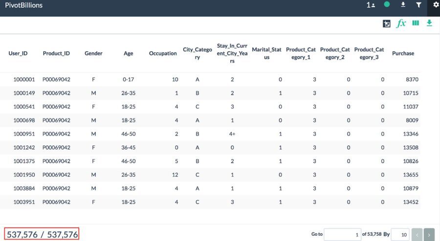
Let’s see what the data looks like. We use Pivot Billions to analyze and manipulate large amounts of data via an intuitive and familiar spreadsheet style. After importing, we see that the data contains over 500K rows at the bottom, along with example data for each column.

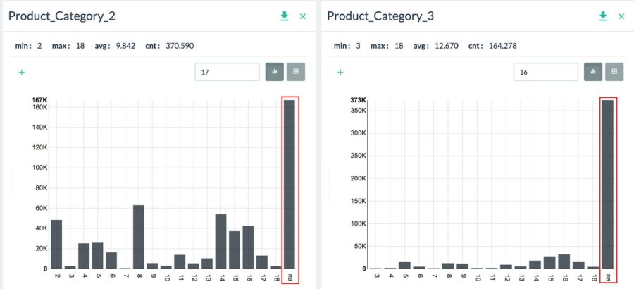
Visualizing the distribution of each column is easy with a simple click of the column name. Overall the data is clean, but Product_Category_2 and Product_Category_3 has many missing values (NAs). They seem like subcategories of Product_Category_1 which has no missing values. Therefore, let’s ignore them for now.

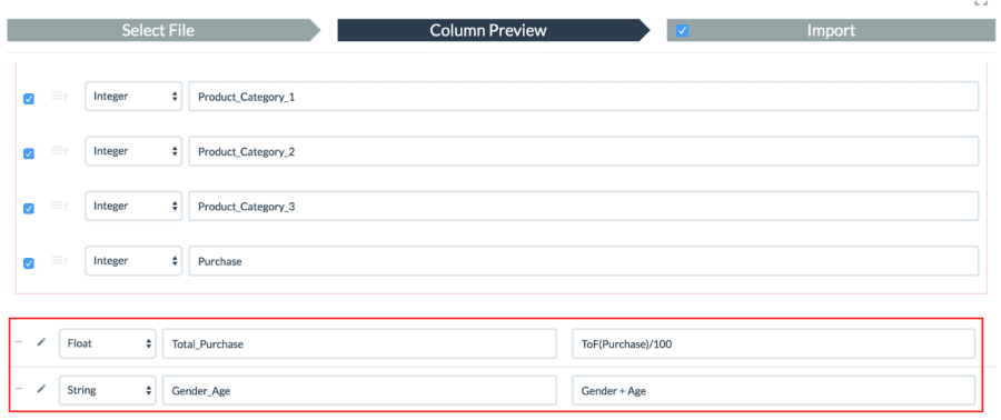
Our next step is preparing data for analysis. First, “Purchase” needs to be divided by 100 to show cents as a decimal point. We define a float column called Total_Purchase and set ToF(Purchase)/100.

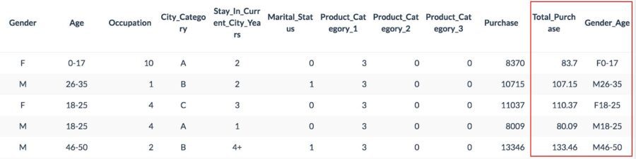
Second, let’s make a column combining gender with age to visualize a bar plot. We define a string column called Gender_Age and then set Gender + Age as the below screenshot.

In Pivot Billions, we can pivot data like Excel. It helps to easily find out the demographics of customers, sales per city, occupation, product category and so on. The bar chart below shows total purchases by product category.

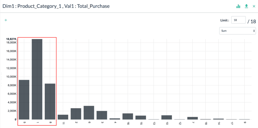
We see that product category 1 is the most popular. It turns out that it generates about 40% of total purchases in this retail chain, and combined purchases from categories 1, 5, and 8 account for more than 70%.

Next, let's examine the data a little more closely! The bar chart below shows total purchases and customer demographics by city.

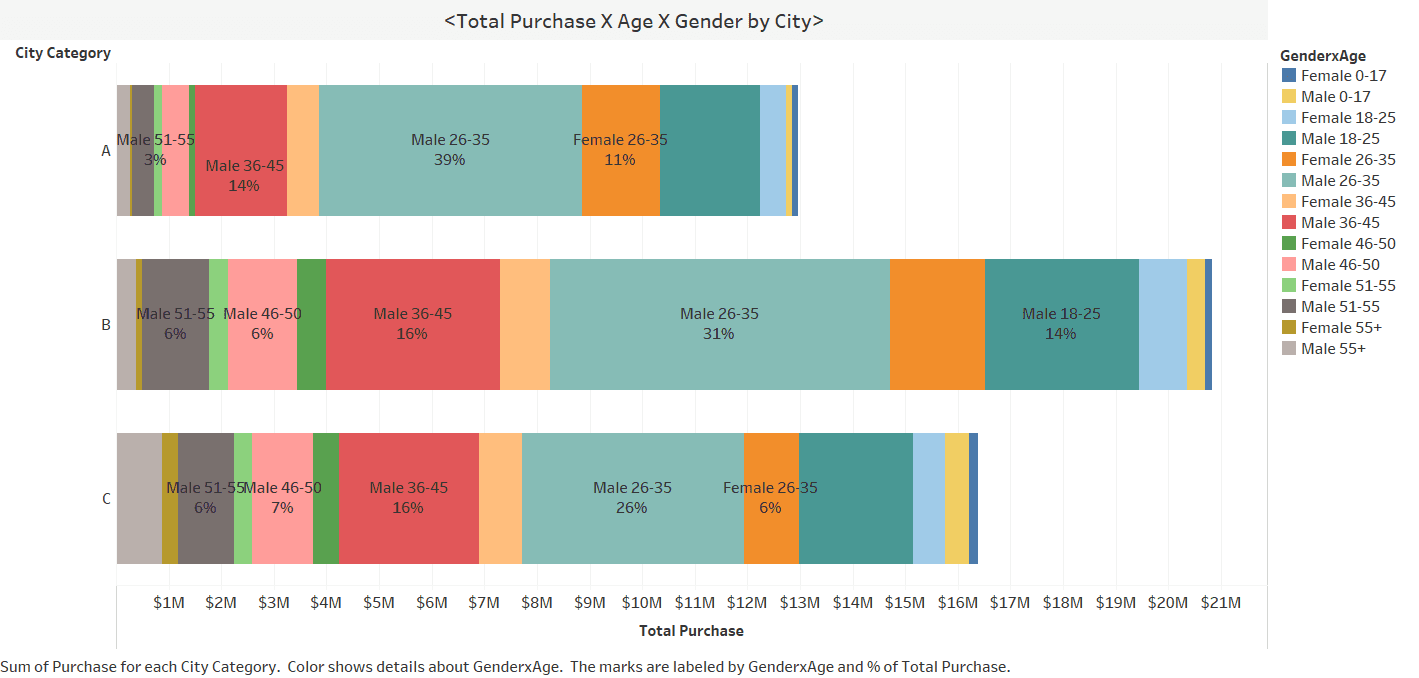
City B has the most sales, and the majority of customers are males ranging in age from the 20’s to 30’s in each city. But City A has a lower ratio of total purchases from customers over 35 compared to the other two cities. City A may have an untapped opportunity to target older demographics in their area. We don’t know each city’s demographics since they’re not revealed in this dataset, but it needs to be considered to understand what causes the differences as a realistic next step. It gives us solid insight for discussing with marketing teams.

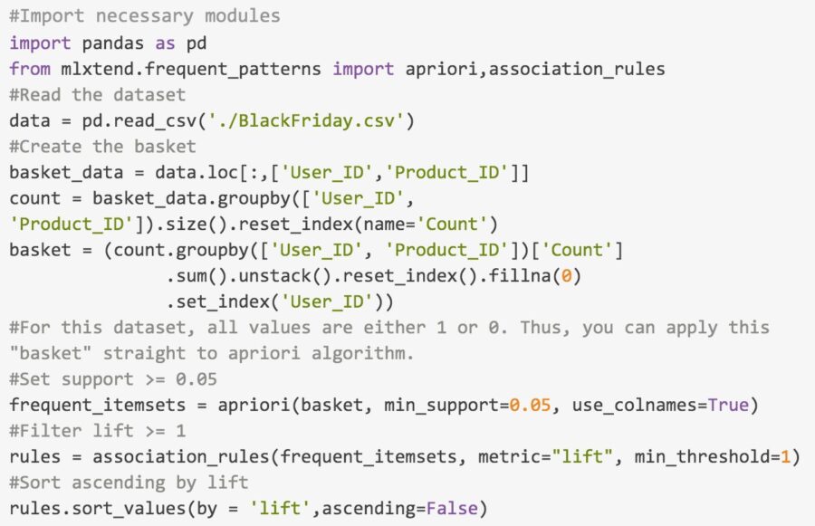
Lastly, let’s do Market Basket Analysis which uses association rule mining on transaction data to discover interesting associations between the products! I’m going to use Apriori algorithm in Python. R also has Apriori algorithm. For further information, please check out the following articles: Apriori(Python), Apriori(R)

We’ll explain briefly what the metrics indicate.

• Support represents how frequently the items appear in the data.
• Confidence represents how frequently the if(antecedents)-then(consequences) statements are found to be true.
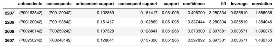
• Lift represents how much larger or smaller confidence than expected confidence is. If a lift is larger than 1.0, it implies that the relationship between the items is more significant than expected.The larger lift means more significant association.

Here’s the result of top 20 lift values by ascending.

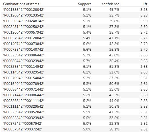
In the Market Basket Analysis, we found strong cross-product purchasing patterns between certain products! These results can be the basis for further analysis or discussion if we are able to know more about the retail chain, and can lead to opportunities for strategic pricing and promotions.