
Who should read this blog:
- Someone who is new to linear regression.
- Someone who wants to understand the jargon around Linear Regression
Code Repository:
https://github.com/DhruvilKarani/Linear-Regression-Experiments
Linear regression is generally the first step into anyone’s Data Science journey. When you hear the words Linear and Regression, something like this pops up in your mind:
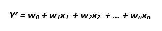
X1, X2, ..Xn are the independent variables or features. W1, W2…Wn are the weights (learned by the model from the data). Y’ is the model prediction. For a set of say 1000 points, we have a table with 1000 rows, n columns for X and 1 column for Y. Our model learns the weights W from these 1000 points so that it can predict the dependent variable Y for an unseen point (a point for which Xs are available but not Y)
For these seen points (1000 in this case), the actual value of the dependent variable (Y) and the model’s prediction of the dependent variable (denoted by Y’) are related as:
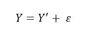
Epsilon (denoted by e henceforth) is the residual error. It captures the difference between models prediction and the actual value of Y. One thing to remember about e is that it follows a normal distribution with 0 mean.
The weights are learned using OLS or Ordinary Least Squared fitting. Meaning, The cumulative squared error, defined as,
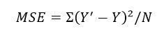
Is minimized. Why do we square the errors and then add? Two reasons.
- If the residual error for a point is -1 and for the other, it is 1 then merely adding them gives 0 error which means the line fits perfectly to the points. This is not true.
- Squaring leads to more importance given to larger errors and less to smaller errors. Intuitively, model weights quickly update to minimize larger errors more than smaller ones.
Quite often, in the excitement of learning new and advanced models, we usually do not fully explore this model. In this blog, we’ll look at how to analyze and diagnose a linear regression model. This blog is going to be as intuitive as possible. Let’s talk about the model. There are three main assumptions linear regression makes:
- The independent variables have a linear relationship with the dependent variable.
- The variance of the dependent variable is uniform across all combinations of Xs
- The error term e associated with Y and Y’ is independent and identically distributed.
Do not worry if you don’t correctly understand the above lines. I am yet to simplify them.
Linear Relationship
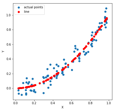
Seems quite intuitive. If the independent variables do not have a linear relationship with the dependent variables, there’s no point modeling them using LINEAR regression. So what should one do if that is not the case? Consider a dataset with one independent variable X and dependent variable Y. In this case, Y varies as the square of X (some random noise is added to Y to make it look more realistic).
If we fit and plot a linear regression line, we can see that it isn’t a good fit. The MSE (mean squared error) is 0.0102
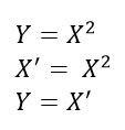
So what we do here is we transform X such that Y and this transformed X follows a linear relationship. Take a look at the picture below. Y and X might not have a linear relation. However, Y and X^2 do have a linear relation.
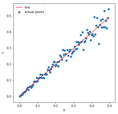
Next, we build the model, generate the predictions and reverse transform it. Take a look at the code and the plots below to get an idea. The MSE here is 0.0053 (almost half the previous one)
Isn’t is evident which one fits better. I hope it is a bit more clear why linear relationships are needed. Let’s move on to the next assumption.
The variance of the dependent variable is uniform across all combinations of Xs
Formally speaking, we need something called homoscedasticity. In simple terms, it means that the residuals must have constant variance. Let’s visualize this. Later I’ll explain why it is essential.
If you notice carefully, the variance among the Y values increases from left to right like a trumpet. Meaning the Y values for lower X values do not vary much concerning the regression line, unlike the ones to the right. We call it heteroscedasticity and is something you want to avoid. Why? Well, if there is a pattern among the residuals, like this one (for the above plot)
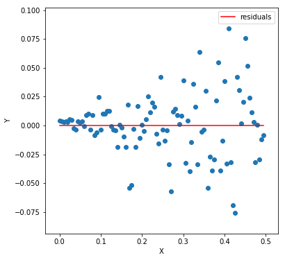
It generally means that the model is too simple for the data. The model is unable to capture all the patterns present in the data. When we achieve homoscedasticity, residuals look something like this. Another reason to avoid heteroscedasticity is to save us from unbias results in significance tests. We’ll look at these tests in details.
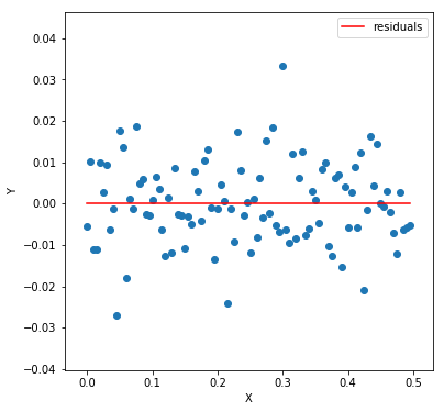
As you can see, the residuals are entirely random. One can hardly see any pattern. Now comes the last and the final assumption.
The error term e associated with Y and Y’ is independent and identically distributed
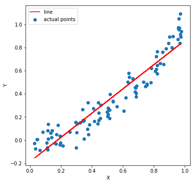
Sounds similar to the previous one? It kind of does. However, it is a little different. Previously, our residuals had growing variance but there we still independent. One residual did not have anything to do with the other. Here, we analyze what if one residual error has some dependency with the other. Consider the following plot whose data is generated by Y = X + noise (random number). Now, this noise accumulates over different values of X. Meaning noise for an X is a random number + the noise of the previous noise. We deliberately introduce this additive noise for the sake of our experiment.
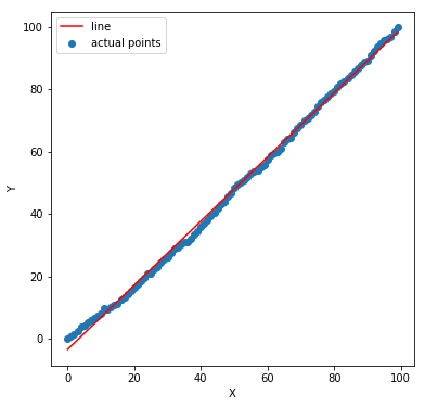
A linear fit seems a good choice. Let’s check the residual errors.

They do not look entirely random. Is there some metric we can compute to validate our claim. It turns out we can calculate something called Autocorrelation. What is autocorrelation? We know that correlation measures the degree of linear relationship between two variables, say A and B. Autocorrelation measures the correlation of a variable with itself. For example, we want to measure how dependent a particular value of A correlates with the value of A some t steps back. More on autocorrelation: https://medium.com/@karanidhruvil/time-series-analysis-3-different-…
In our example, it turns out to be 0.945 which indicates some dependency. Now, why do we need errors to be independent? Again, this means the linear model fails to capture complex patterns in the data. Such type of patterns may frequently occur in time series data (where X is time, and Y is a property that varies with time. Stock prices for instance). The unaccounted patterns here could be some seasonality or trends.
I hope the three assumptions are a bit clear. Now how do we evaluate our model? Let’s take a look at some metrics.
Evaluating a Model
Previously, we defined MSE to calculate the errors committed by the model. However, if I tell you that for some data and some model the MSE is 23.223. Is this information alone enough to say something about the quality of our fit? How do we know if it’s the best our model can do? We need some benchmark to evaluate our model against. Hence, we have a metric called R squared (R^2).
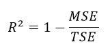
Let’s get the terms right. We know MSE. However, what is TSE or Total Squared Error? Suppose we had no X. We have Y, and we asked to model a line to fit these Y values such that the MSE minimizes. Since we have no X, our line would be of the form Y’ = a, where a is a constant. If we substitute Y’ for a in the MSE equation, and minimize it by differentiating with respect to a and set equal to zero, it turns out that a = mean(Y) gives the least error. Think about this – the line Y’ = a can be understood as the baseline model for our data. Addition of any independent variable X improves our model. Our model cannot be worse than this baseline model. If our X didn’t help to improve the model, it’s weight or coefficients would be 0 during MSE minimization. This baseline model provides a reference point. Now come back to R squared and take a look at the expression. If our model with all the X and all the Y produces an error same as the baseline model (TSE), R squared = 1-1 = 0. This is the worst case. On the opposite, if MSE =0, R squared = 1 which is the best case scenario.
Now let’s take a step back and think about the case when we add more independent variables to our data. How would the model respond to it? Suppose we are trying to predict house prices. If we add the area of the house to our model as an independent variable, our R square could increase. It is obvious. The variable does affect house prices. Suppose we add another independent variable. Something garbage, say random numbers. Can our R square increase? Can it decrease?
Now, if this garbage variable is helping minimize MSE, it’s weight or coefficient is non zero. If it isn’t, the weight is zero. If so, we get back the previous model. We can conclude that adding new independent variable at worst does nothing. It won’t degrade the model R squared. So if I keep adding new variables, I should get a better R squared. And I will. However, it doesn’t make sense. Those features aren’t reliable. Suppose if those set of random numbers were some other set of random numbers, our weights would change. You see, it is all up to chance. Remember that we have a sample of data points on which we build a model. It needs to be robust to new data points out of the sample. That’s why we introduce something called adjusted R squared. Adjusted R squared penalizes any addition of independent variables that do not add a significant improvement to the model. You usually use this metric to compare models after the addition of new features.
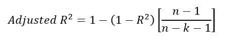
n is the number of points, k is the number of independent variables. If you add features without a significant increase in R squared, the adjusted R squared decreases.
So now we know something about linear regression. We dive deeper in the second part of the blog. In the next blog, we look at regularization and assessment of coefficients.
Read more here.