

Here, we introduce Bass diffusion model which is a classic way to predict sales for newly launched product in the market. It is an effective way to know the overall sales of the product in its lifecycle and make strategy accordingly.
After launching a new product in the market, sales prediction for it has always been a difficult task due to lack of historical data. However, having an accurate prediction is extremely important not only from a marketing standpoint, but also for managing overall product life cycle. It helps in making overall strategy for the product like determining the time for markdown, promotion and introduction of an updated version of the product in the market.
Bass diffusion model is a classic model for this purpose and it has successfully been used for sales prediction of many such new products very accurately. It consists of some simple differential equations describing the process of how a product gets adopted in the market.
The model makes two basic assumptions about the potential buyers:
- When a product is introduced in the market, there are some customers who buy the product only based on external communication like mass media advertisements and without the influence of any person. They are the early adopter of the product and are called Innovators.
- The other set of customers are first influenced by the Innovators, gets the review from them and only then purchase the product. These set of customers are called Imitators.
The other assumptions are:
- The overall market size is fixed
- All the customers in the market will eventually buy the product
- No repeat purchase is happening
Next, let’s have a look at the equations first and formulate them:
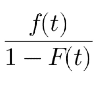
Let’s define the cumulative probability of a customer buying the product till time t is F(t). Then the probability of purchase for that customer at time t is f(t) = F´(t). The rate of purchase at time t is:
Which basically signifies the ratio between probability of purchasing the product at time t given that the customer has not bought it till time t.
As per Bass, this purchase rate can be defined as:
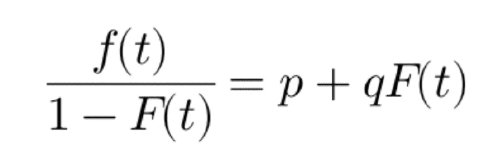
Where p is the rate of innovative adoption and q is imitation rate. Further, q is multiplied by F(t) as imitation can happen only based on the current innovative adoption. So, the above equation gives probability of total adoption by a customer at time t, both from innovative adoption and imitation adoption.
Now, if we solve the equation, we get as follows (If you are not interested in Maths, you can skip this part and jump to the final values for f(t) and F(t)):
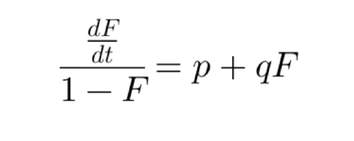
From t = 0, we get,
F(0) = 0 and
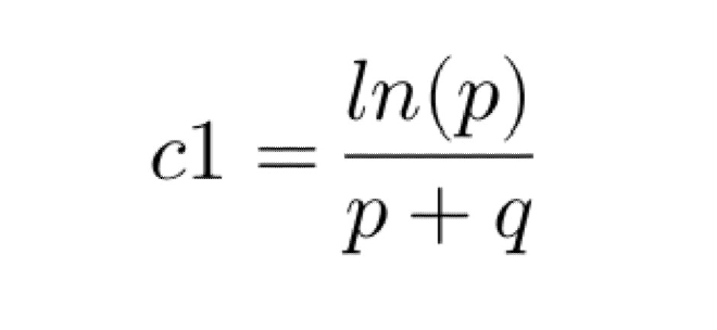
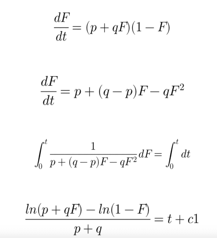
Substituting the above in the main equation and solving for F(t), we get,
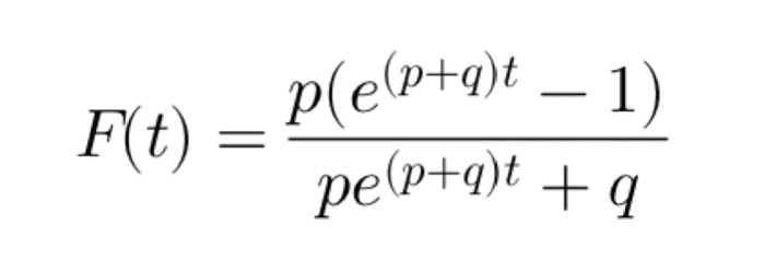
And, f(t) will be,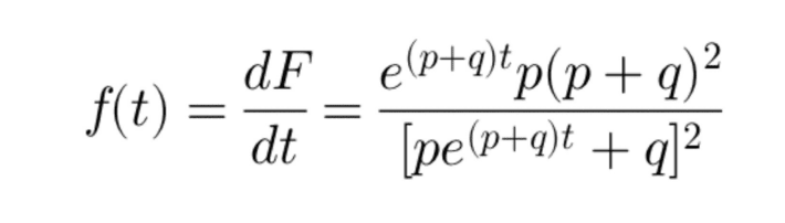
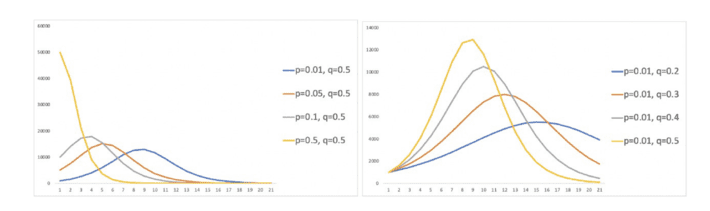
Also, if the total market size is m, then the total adoption at time t will be m*f(t). Below are the sales curves for different values of p and q considering the market size to be fixed at 100,000. Usually, in real life, p is smaller than q.
Now, the immediate next question is how to estimate p, q and m. It can be estimated from first few week’s sales of the product or past sales of similar product (eg older version of the product or product category). Here, we will see how we can obtain the estimate using OLS. However, the same can also be obtained using NLS.
If the market size is m then total sales in any period is given by,
s(t) = m*f(t)
And cumulative sales up to time t is S(t) = m*F(t). From Bass equation, we get,
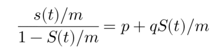
With simple algebraic calculation, the above can be re-written as:
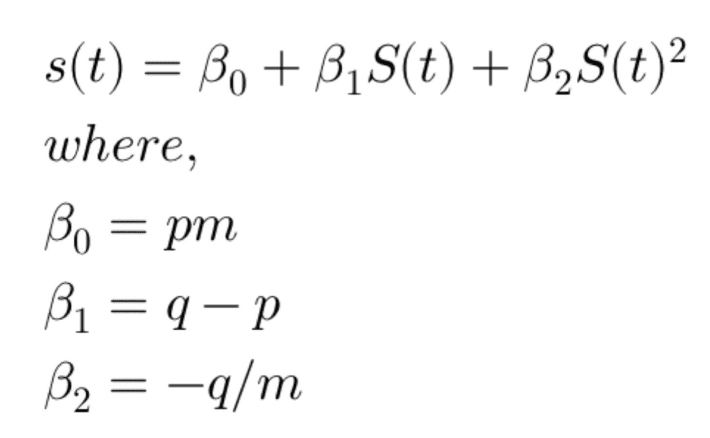
So, the Bass equation essentially becomes a regression of sales at time t on cumulative sales till time t. And the coefficients β0, β1 and β2 can easily be estimated using OLS. Once, the estimation is done, p, q and m can be back calculated from the coefficients as below: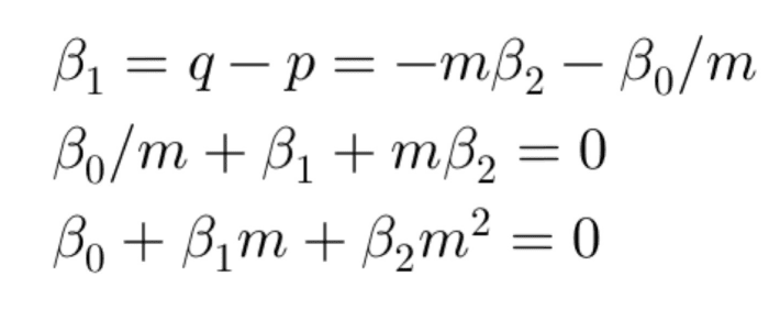
The above is a quadratic equation in m and can easily be solved to get a value for m in terms of β0, β1 and β2. Substituting the value of m in p = β0/m and q = -mβ2, we can also get the value for p and q.
Although, it is an excellent method of predicting sales of a newly introduced product in the market and has been used for many use cases in past, there are some limitations of it:
- The model assumes a particular shape of sales over time. This might not be true at a very granular level, for example, daily sales prediction
- Coefficient estimation of the model needs some past data of the product. However, it might be too late for the business to take any decision by the time the data is available
- If the data considered is not reliable, the estimation and in turn the prediction becomes unreliable
- The model assumes that the market is fixed which is often not the case due to price change, promotion and other business activities.
- The model does not take into account the repeat purchases of the customers.
- The model does not take into account the cannibalization or any impact of other products available in the market
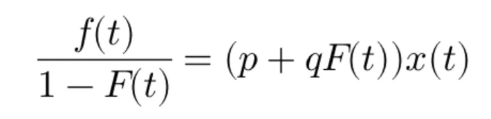
To overcome the above limitations, lots of researches have been conducted and the model has been extended to accommodate some of the other factors affecting sales. Like the below one takes into account the price and other features of the product (denoted by x(t)):
In conclusion, in the article, we saw how Bass diffusion model can be used to estimate sales of a new product in the market, how to estimate the coefficients and some of its limitations. This is a well researched model and lots of extensions of the model are also available. The key issue, however, is the estimation of the coefficients. Nevertheless, the model can still give a fair prediction of sales which can be used for many business decisions regarding the product strategy.