
This article was posted by S. Richter-Walsh.
A Brief Introduction:
Linear regression is a classic supervised statistical technique for predictive modelling which is based on the linear hypothesis:
y = mx + c
where y is the response or outcome variable, m is the gradient of the linear trend-line, x is the predictor variable and c is the intercept. The intercept is the point on the y-axis where the value of the predictor x is zero.
In order to apply the linear hypothesis to a dataset with the end aim of modelling the situation under investigation, there needs to be a linear relationship between the variables in question. A simple scatterplot is an excellent visual tool to assess linearity between two variables. Below is an example of a linear relationship between miles per gallon (mpg) and engine displacement volume (disp) of automobiles which could be modelled using linear regression. Note that there are various methods of transforming non-linear data to make them appear more linear such as log and square root transformations but we won’t discuss those here.
attach(mtcars)
plot(disp, mpg, col = “blue”, pch = 20)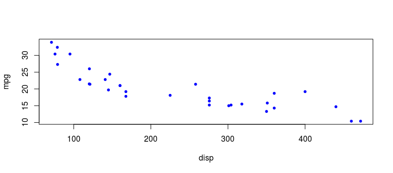
Now, in order to fit a good model, appropriate values for the intercept and slope must be found. R has a nice function, lm(), which creates a linear model from which we can extract the most appropriate intercept and slope (coefficients).
model <- lm(mpg ~ disp, data = mtcars)
coef(model)
(Intercept) disp
29.59985476 -0.04121512
We see that the intercept is set at 29.59985476 on the y-axis and that the gradient is -0.04121512. The negative gradient tells us that there is an inverse relationship between mpg and displacement with one unit increase in displacement resulting in a 0.04 unit decrease in mpg.
How are these intercept and gradient values calculated one may ask? In finding the appropriate values, the goal is to reduce the value of a statistic known as the mean squared error (MSE):
MSE = Σ(y – y_preds)² / n
where y represents the observed value of the response variable, y_preds represents the predicted y value from the linear model after plugging in values for the intercept and slope, and n is the number of observations in the dataset. Each set of xy data points are iterated over to find the squared error, all squared errors are summed and the sum is divided by n to get the MSE.
Using the linear model we created earlier, we can obtain y predictions and plot them on the scatterplot as a regression line. We use the predict() function in base R and plot the predicted values using abline().
y_preds <- predict(model)
abline(model)
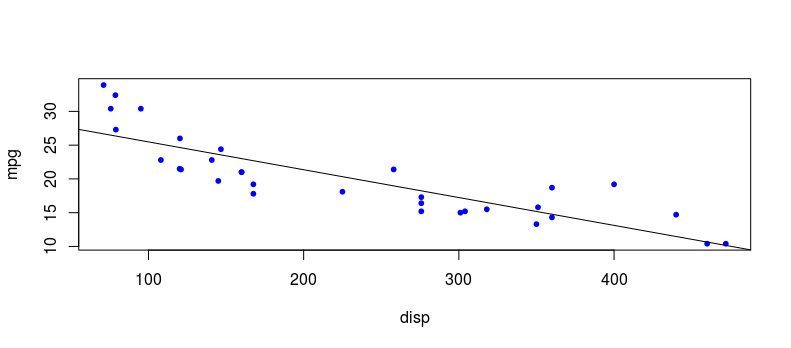
Next, we can calculate the MSE by summing the squared differences between observed yvalues and our predicted y values then dividing by the number of observations n. This gives a MSE of 9.911209 for this linear model.
errors <- unname((mpg – y_preds) ^ 2)
sum(errors) / length(mpg)
To read the full article, click here.
Top DSC Resources
- Article: What is Data Science? 24 Fundamental Articles Answering This Question
- Article: Hitchhiker’s Guide to Data Science, Machine Learning, R, Python
- Tutorial: Data Science Cheat Sheet
- Tutorial: How to Become a Data Scientist – On Your Own
- Categories: Data Science – Machine Learning – AI – IoT – Deep Learning
- Tools: Hadoop – DataViZ – Python – R – SQL – Excel
- Techniques: Clustering – Regression – SVM – Neural Nets – Ensembles – Decision Trees
- Links: Cheat Sheets – Books – Events – Webinars – Tutorials – Training – News – Jobs
- Links: Announcements – Salary Surveys – Data Sets – Certification – RSS Feeds – About Us
- Newsletter: Sign-up – Past Editions – Members-Only Section – Content Search – For Bloggers
- DSC on: Ning – Twitter – LinkedIn – Facebook – GooglePlus
Follow us on Twitter: @DataScienceCtrl | @AnalyticBridge