Implementing a Soft-Margin Kernelized Support Vector Machine Binary Classifier with Quadratic Programming in R and Python

In this article, couple of implementations of the support vector machine binary classifier with quadratic programming libraries (in R and python respectively) and application on a few datasets are going to be discussed.

The next figure describes the basics of Soft-Margin SVM (without kernels).
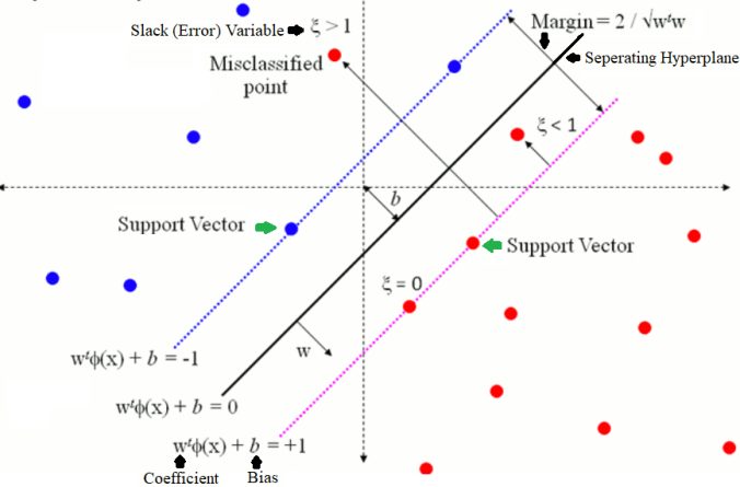SVM in a nutshell

Given a (training) dataset consisting of positive and negative class instances.
Objective is to find a maximum-margin classifier, in terms of a hyper-plane (the vectors w and b) that separates the positive and negative instances (in the training dataset).
If the dataset is noisy (with some overlap in positive and negative samples), there will be some error in classifying them with the hyper-plane.
In the latter case the objective will be to minimize the errors in classification along with maximizing the margin and the problem becomes a soft-margin SVM (as opposed to the hard margin SVM without slack variables).
A slack variable per training point is introduced to include the classification errors (for the miss-classified points in the training dataset) in the objective, this can also be thought of adding regularization.
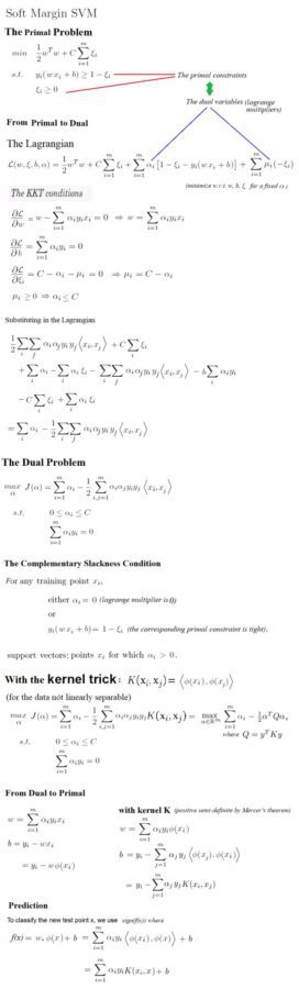
The optimization problem is quadratic in nature, since it has quadratic objective with linear constraints.
It is easier to solve the optimization problem in the dual rather than the primalspace, since there are less number of variables.
Hence the optimization problem is often solved in the dual space by converting the minimization to a maximization problem (keeping in mind the weak/strong duality theorem and the complementary slackness conditions), by first constructing the Lagrangian and then using the KKT conditions for a saddle point.
If the dataset is not linearly separable, the kernel trick is used to conceptually map the datapoints to some higher-dimensions only by computing the (kernel) gram matrix / dot-product of the datapoints (the matrix needs to positive semi-definite as per Mercer’s theorem).
Some popular kernel functions are the linear, polynomial, Gaussian (RBF, corresponding to the infinite dimensional space) kernels.
The dual optimization problem is solved (with standard quadratic programmingpackages) and the solution is found in terms of a few support vectors (defining the linear/non-liear decision boundary, SVs correspond to the non-zero values of the dual variable / the primal Lagrange multipler), that’s why the name SVM.
Once the dual optimization problem is solved , the values of the primal variables are computed to construct the hyper-plane / decision surface.
Finally the dual and primal variables (optimum values obtained from the solutions) are used in conjunction to predict the class of a new (unseen) datapoint.
The hyper-parameters (e.g., C) can be tuned to fit different models.

The following figure describes the soft-margin SVM in a more formal way.

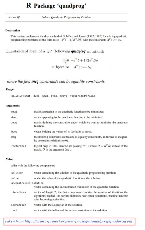
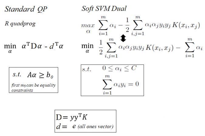
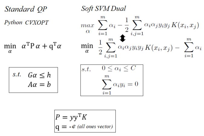
The following figures show how the SVM dual quadratic programming problem can be formulated using the R quadprog QP solver (following the QP formulation in the R package quadprog).

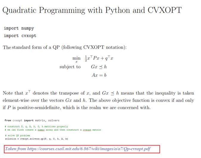
The following figures show how the SVM dual quadratic programming problem can be formulated using the Python CVXOPT QP solver (following the QP formulation in the python library CVXOPT).

The following R code snippet shows how a kernelized (soft/hard-margin) SVM model can be fitted by solving the dual quadratic optimization problem.

library(quadprog)
library(Matrix)
 
svm_fit <- function(X, y, FUN=linear_kernel, C=NULL) {
 n_samples <- nrow(X)
 n_features <- ncol(X)
 # Gram matrix
 K <- matrix(rep(0, n_samples*n_samples), nrow=n_samples)
 for (i in 1:n_samples){
  for (j in 1:n_samples){
   K[i,j] <- FUN(X[i,], X[j,])
  }
 }
 Dmat <- outer(y,y) * K
 # convert Dmat to the nearest positive definite matrix
 Dmat <- as.matrix(nearPD(Dmat)$mat)
 dvec <- rep(1, n_samples)
 if (!is.null(C)) { # soft-margin
  Amat <- rbind(y, diag(n_samples), -1*diag(n_samples))
  bvec <- c(0, rep(0, n_samples), rep(-C, n_samples))
 } else {           # hard-margin
  Amat <- rbind(y, diag(n_samples))
  bvec <- c(0, rep(0, n_samples))
 }
 res <- solve.QP(Dmat,dvec,t(Amat),bvec=bvec, meq=1)
 # Lagrange multipliers
 a <- res$solution
 # Support vectors have non zero lagrange multipliers
 ind_sv  1e-5) # some small threshold
# ...
}

The following python code from Mathieu Blondel’s Blog, shows how a kernelized (soft/hard-margin) SVM model can be fitted by solving the dual quadratic optimization problem.

import numpy as np
import cvxopt
def fit(X, y, kernel, C):
    n_samples, n_features = X.shape
    # Compute the Gram matrix
    K = np.zeros((n_samples, n_samples))
    for i in range(n_samples):
       for j in range(n_samples):
           K[i,j] = kernel(X[i], X[j])
    # construct P, q, A, b, G, h matrices for CVXOPT
    P = cvxopt.matrix(np.outer(y,y) * K)
    q = cvxopt.matrix(np.ones(n_samples) * -1)
    A = cvxopt.matrix(y, (1,n_samples))
    b = cvxopt.matrix(0.0)
    if self.C is None: # hard-margin SVM
       G = cvxopt.matrix(np.diag(np.ones(n_samples) * -1))
       h = cvxopt.matrix(np.zeros(n_samples))
    else:              # soft-margin SVM
       G = cvxopt.matrix(np.vstack((np.diag(np.ones(n_samples) * -1), np.identity(n_samples))))
       h = cvxopt.matrix(np.hstack((np.zeros(n_samples), np.ones(n_samples) * C)))
    # solve QP problem
    solution = cvxopt.solvers.qp(P, q, G, h, A, b)
    # Lagrange multipliers
    a = np.ravel(solution['x'])
    # Support vectors have non zero lagrange multipliers
    sv = a > 1e-5 # some small threshold
    # ...

Notes

Since the objective function for QP is convex if and only if the matrix P (in python CVXOPT) or Dmat (in R quadprog) is positive-semidefinite, it needs to be ensured that the corresponding matrix for SVM is psd too.
The corresponding matrix is computed from the Kernel gram matrix (which is psd or non-negative-definite by Mercer’s theorem) and the labels from the data. Due to numerical errors, often a few eigenvalues of the matrix tend to be very small negative values.
Although python CVXOPT will allow very small numerical errors in P matrix with a warning message, R quardprog will strictly require that the Dmat matrix is strictly positive definite, otherwise it will fail.
Hence, with R quadprog the D matrix first needs to be converted to a positive definite matrix using some algorithm (particularly in case when it contains very small negative eigenvalues, which is quite common, since D comes from the data).
Cases corresponding to the hard and soft-margin SVMs must be handled separately, otherwise it will lead to inconsistent system of solutions.

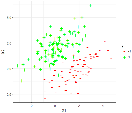
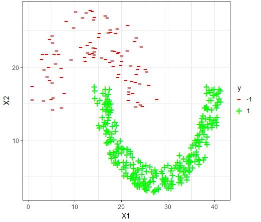
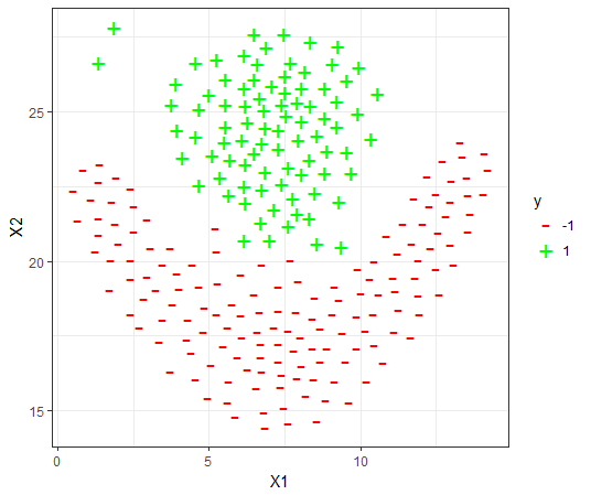
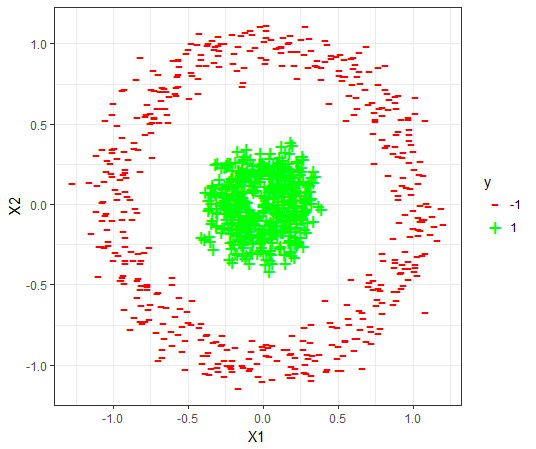
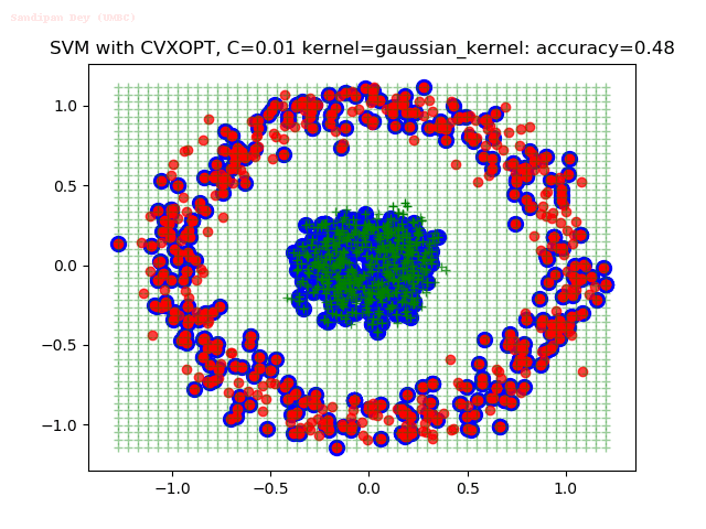
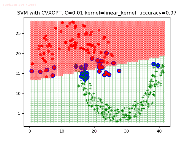
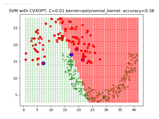
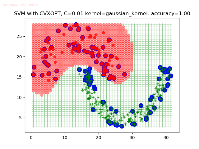
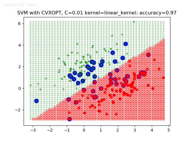
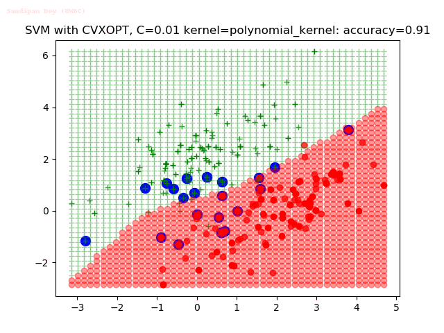
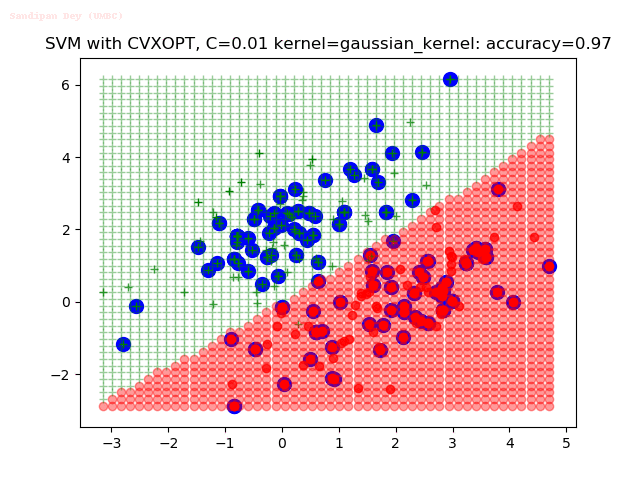
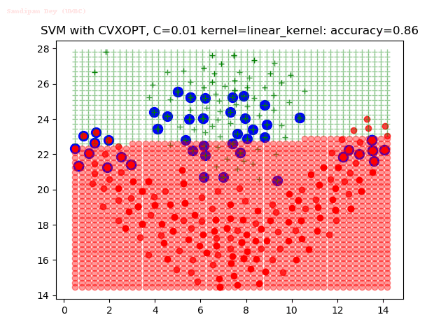
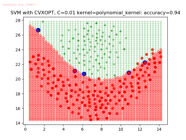
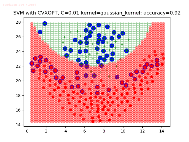
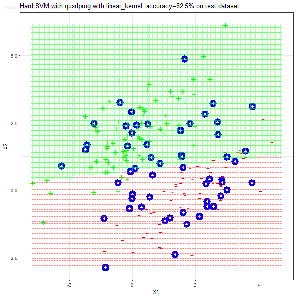
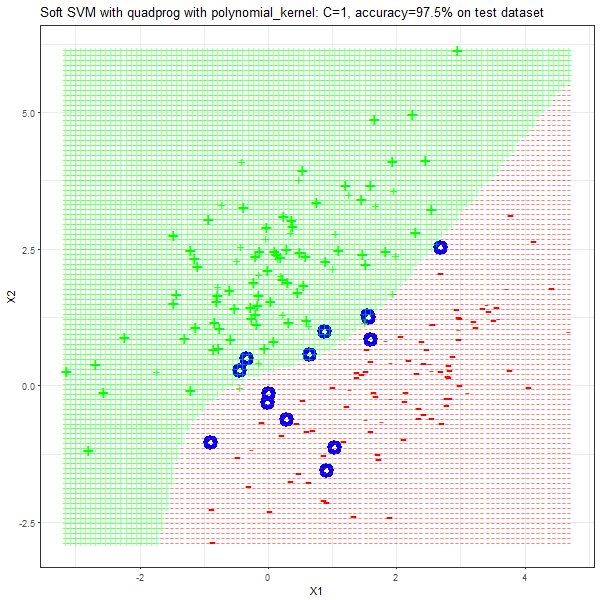
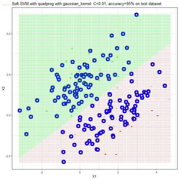
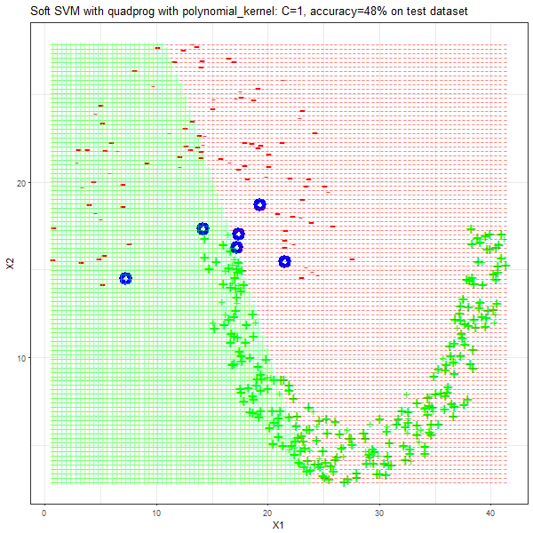
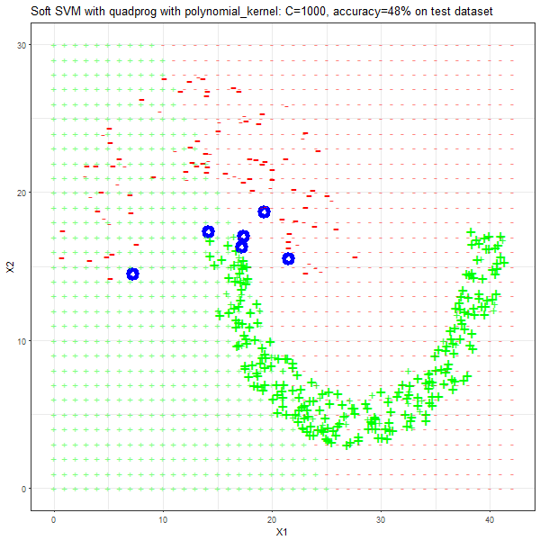
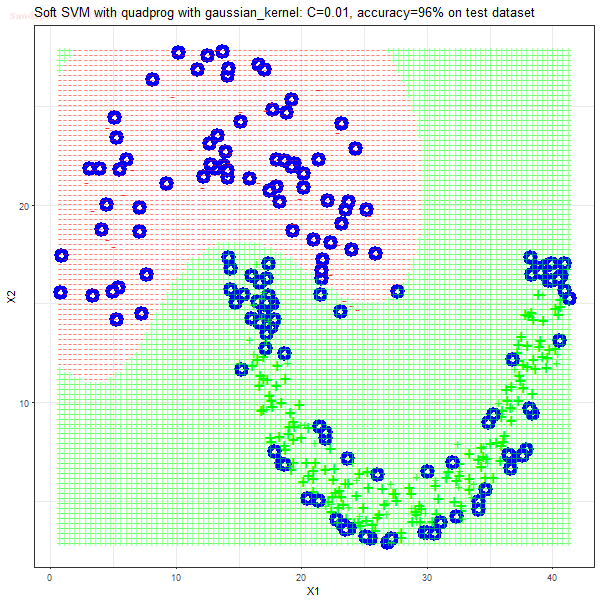
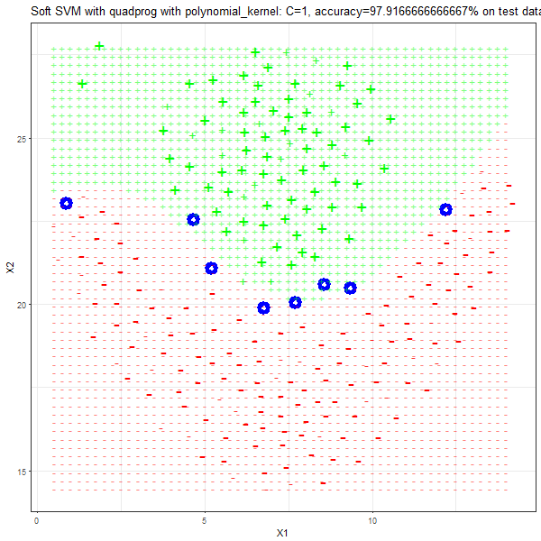
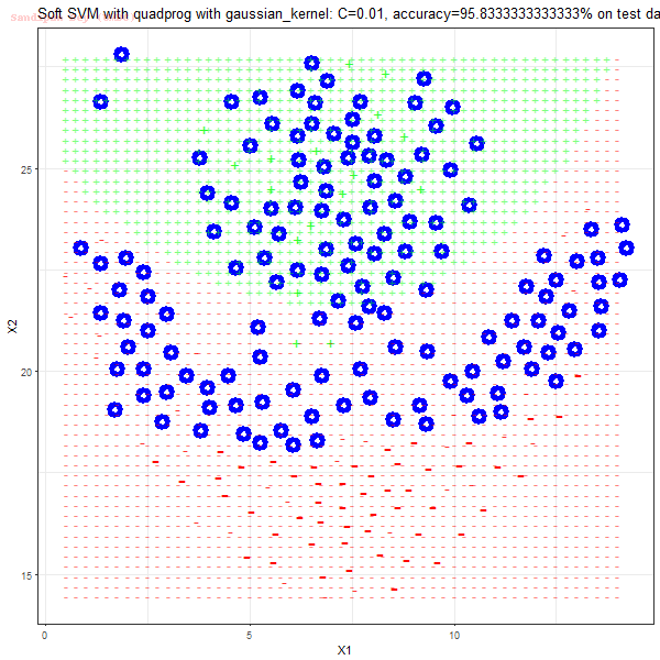
Using the SVM implementations for classification on some datasets

The datasets

For each dataset, the 80-20 Validation on the dataset is used to

First fit (train) the model on randomly selected 80% samples of the dataset.
Predict (test) on the held-out (remaining 20%) of the dataset and compute accuracy.
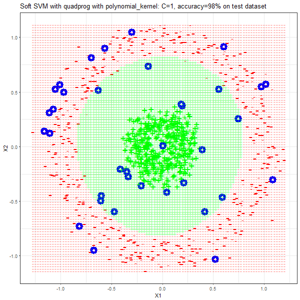
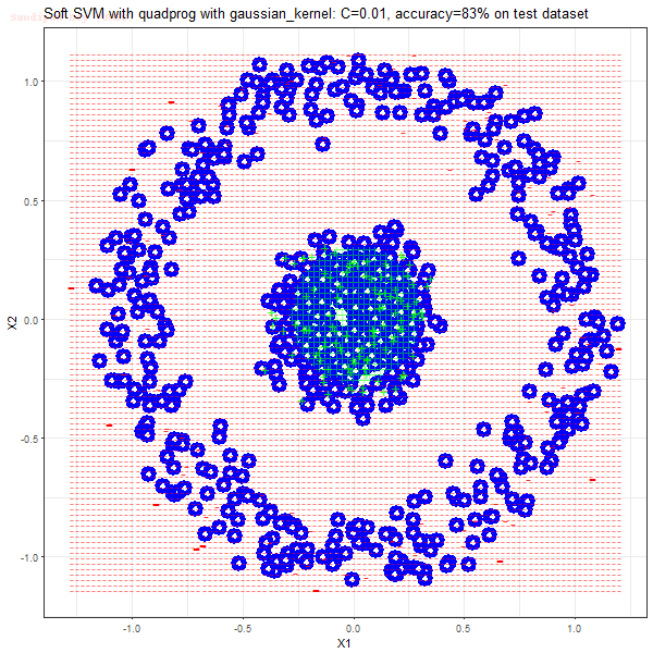
Different values of the hyper-parameter C and different kernels are used.
For the polynomial kernel, polynomial of degree 3 is used and the RBF kernel with the standard deviation of 5 is used, although these hyper-parameters can be tuned too.

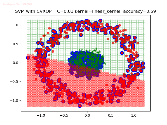
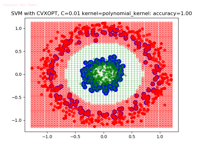
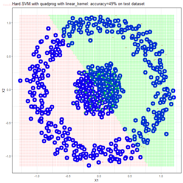
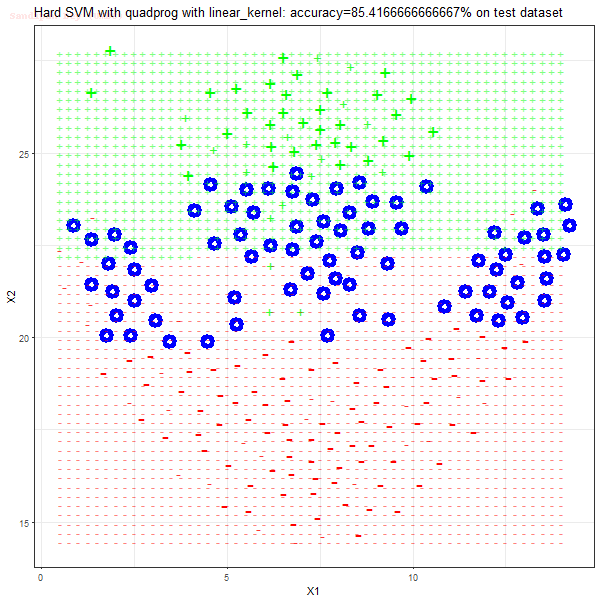
Results

As can be seen from the results below,

The points with blue circles are the support vectors.
When the C value is low (close to hard-margin SVM), the model learnt tends to overfit the training data.
When the C value is high (close to soft-margin SVM), the model learnt tends to be more generalizable (C acts as a regularizer).
There are more support vectors required to define the decision surface for the hard-margin SVM than the soft-margin SVM for datasets not linearly separable.
The linear (and sometimes polynomial) kernel performs pretty badly on the datasets that are not linearly separable.
The decision boundaries are also shown.