
While many of the programming libraries encapsulate the inner working details of graph and other algorithms, as a data scientist it helps a lot having a reasonably good familiarity of such details. A solid understanding of the intuition behind such algorithms not only helps in appreciating the logic behind them but also helps in making conscious decisions about their applicability in real life cases. There are several graph based algorithms and most notable are the shortest path algorithms. Algorithms such as Dijkstra’s, Bellman Ford, A*, Floyd-Warshall and Johnson’s algorithms are commonly encountered. While these algorithms are discussed in many text books and informative resources online, I felt that not many provided visual examples that would otherwise illustrate the processing steps to sufficient granularity enabling easy understanding of the working details. As such, I had to use simple enough graphs to visualize the algorithmic flow for my own understanding and I wanted to share my examples along with the explanations through this article. Since there are many algorithms to illustrate, I decided to divide the article into several parts. In part 1, I have illustrated Dijkstra’s and Bellman-Ford algorithms. Before diving into algorithms, I also wanted to highlight salient points on the graph data structure.
Quick Primer On Graph Data Structure
A graph is a data structure comprising of a finite non-empty set of vertices wherein some pairs of vertices are connected. In real life, such vertices represent real world objects wherein some pairs of such objects are related and such relationship is represented by a link connection. The link between a pair of vertices is referred to as an edge. Edges have directionality. In case of unidirectional edge, an arrow points from the tail vertex (source) to the head vertex (target) and hence link goes one way. As such, an edge between vertices v1 and v2 is an ordered pair (v1, v2) where v1 is the tail vertex and v2 is the head vertex. In case of a bidirectional edge, arrows point in both the directions and hence link goes both ways. As such, an edge between vertices v1 and v2 is unordered pair wherein both (v1, v2) and (v2, v1) represent the same edge. A graph which contains all unidirectional edges is called as a directed graph. A graph which contains all bidirectional edges is called as undirected graph. A graph in which some edges are unidirectional and some are bidirectional is called as mixed graph. The number of edges incident to a vertex is called as the degree of the vertex. The out-degree of a vertex is the number of directed edges incident to the vertex where the vertex is the tail and the in-degree of a vertex is the number of directed edges incident to the vertex where the vertex is the head. In addition, edges have weights. Edge weight represents the capacity or cost or distance of that edge. As such, edge weight can be positive or negative number. A path from vertex v1 to vertex vn is a sequence of vertices v1, v2, v3…vn in a graph such that the pairs (v1, v2), (v2, v3)…(vn-1, vn) are connected via edges in the graph. As such, two vertices are connected if a path exists between them in the graph. A path is said to be simple if all the vertices are distinct with the exception of the first and the last vertices. A path is said to be circular or cyclic if the first and the last vertex are same. A directed graph without any circular paths is called as Directed Acyclic Graph (DAG). The number of edges in a path represents the path’s length and the sum of the edge weights in the path represents the capacity or cost or distance of that path. If the path weight is negative in a cyclic path, then that path is referred to as negative cycle.
A graph is said to be complete if each of its vertices is connected to all other vertices. If there are N vertices in a complete graph, then there will be N(N-1)/2 edges in the graph. Complete graphs are also commonly referred to as universal graphs.
Dijkstra’s Algorithm
Dijkstra’s algorithm is a greedy algorithm used to find the shortest path between a source vertex and other vertices in a graph containing weighted edges. An algorithm is said to be greedy if it leverages local optimal solution at every step in its execution with the expectation that such local optimal solution will ultimately lead to global optimal solution. As such, Dijkstra’s algorithm works on a greedy expectation that a sub-path between vertices A and B within a global shortest path between vertices A and C, is also a shortest path between A and B. The limitation in Dijkstra’s algorithm is that it may not work if there are negative edge weights and definitely will not work if there are negative cycles in the graph. The algorithm measures the shortest path from the source vertex to all other vertices by visiting a source vertex, measuring the path lengths from the source to all its neighboring vertices and then visiting one of the neighbors with the shortest path. Algorithm repeats these steps iteratively until it completes visiting all vertices in the graph.
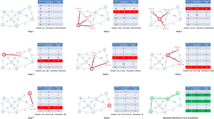
Figure 1: Illustrations of Dijkstra’s Algorithm
Figure 1 illustrates the logical steps in the execution of Dijkstra’s algorithm. The algorithm starts with maintaining two sets; 1] a set with all unvisited vertices and 2] a set with all visited vertices which is initially empty. In addition, the algorithm maintains a tally of tentative shortest paths for each vertex in the graph measured thus far from the source vertex and keeps a reference to a predecessor vertex on the path to each vertex from the source vertex. As shown in figure 1, at step 1, the algorithm sets the distances from the source vertex, A in the example, to rest of the vertices as infinity and the distance from the source to itself as 0. At step 2, the algorithm measures the tentative distances to each of the unvisited neighbors of source vertex, B, C and E in the example. A distance of a vertex from the source is considered as tentative until algorithm confirms it to be the shortest distance. Tentative distance of vertex V, given the tentative distance of vertex U from the source, is measured using the formula d(U) + d(U,V) where d(U) is the tentative distance of vertex U from the source vertex and d(U,V) is the edge weight between vertices U and V. If newly measured tentative distance, i.e., d(U) + d(U,V), is less than the previously assigned tentative distance of vertex V, d(V), then the algorithm updates tentative distance of vertex V with the new value, i.e., d(V) = d(U) + d(U,V). This process of updating vertex distance if the newly measured distance is less than the previously assigned distance is commonly referred to as relaxation. If a vertex’s distance gets updated with newly measured distance lesser than its previous measured distance, then the vertex is considered as relaxed. In the example, algorithm relaxes vertices B, C and E and at the same time sets vertex A as their predecessor vertex. The algorithm marks the current source vertex A as visited, pops it out of the unvisited set and places it in the visited set. The algorithm then determines the neighbor vertex with shortest distance as the next vertex to be visited, vertex C in the example, and iterates to the next step. At step 3, the algorithm measures the tentative distances of unvisited neighbors of vertex C, i.e., B, D and E, relative to the original source vertex A. The algorithm relaxes vertex D with new tentative distance and sets its predecessor path vertex as C. The algorithm does not update the tentative distances of vertices B and E since their distances measured via vertex C are greater than their previously assigned tentative distances. As in step 2, the algorithm marks the current vertex C as visited, pops it out of the unvisited set and places it in the visited set. The algorithm then determines the unvisited vertex with the shortest distance as the next vertex to be visited, vertex B in the example, and iterates to the next step. Algorithm will repeat such steps until all the vertices have been marked as visited or there are no more connected vertices to evaluate. The shortest path from source vertex to any other vertex can then be determined by looking up the predecessor vertices from the evaluated table. For example, to determine the shortest path from vertex A to vertex G, table can be looked up to find the predecessor vertex of G which is D. The predecessor vertex of D is B and the predecessor vertex of B is A. As such, the shortest path from vertex A to vertex G is {A,B,D,G} with a shortest distance of 11.
In a complete graph comprising of N vertices, where each vertex is connected to all other vertices, the number of vertices to be visited by the algorithm will be N. Also the number of vertices potentially relaxed each time a vertex is visited is also N. As such, the worst case time complexity of Dijkstra’s algorithm is in the order of NxN = N2.
Bellman-Ford Algorithm
Bellman-Ford algorithm is used to find the shortest paths from a source vertex to all other vertices in a weighted graph. Unlike Dijkstra’s algorithm, Bellman-Ford algorithm can work when there are negative edge weights. The core of the algorithm is centered on iteratively relaxing the path distances of vertices from the source vertex. If there are N vertices, the maximum number of edges from the source vertex to the Nth vertex could possibly be (N-1) edges. As such, the algorithm iterates utmost (N-1) times to relax the vertex distances. In every iteration, the algorithm starts at the source vertex, walks the outgoing edges to the connected neighbors and evaluates the tentative distance of each of the neighbors and updates the tentative distance if it is less than the previous value. The algorithm then moves to next vertex and repeats the process of walking the outgoing edges and accordingly relaxing the tentative distances for each of the connected neighbors. As such, in every iteration, the algorithm visits all the vertices and walks all the edges thereby relaxing the vertex distances wherever possible. The algorithm repeats the iterations of relaxing the vertices utmost (N-1) times or until no vertices can be updated anymore.
 Figure 2: Illustrations of Bellman-Ford Algorithm
Figure 2 illustrates the logical steps in the execution of Bellman-Ford algorithm. In essence, the algorithm maintains a table containing the evaluated shortest distances to each of the vertices from the source vertex along with the predecessor vertex, which would get updated potentially at every iteration. In the example graph, there are 4 vertices and hence the algorithm will execute utmost 4-1 = 3 iterations. At the initiation step, the algorithm sets the distances from the source vertex, A in the example, to all other vertices as infinity and the distance from source vertex to itself as 0 in the table. At this step, the predecessor vertex row is empty. The algorithm then begins iteration 1. The algorithm starts at the source vertex and evaluates the distances to the neighbors connected by outgoing edges. In the example, vertex A has only one outgoing edge to vertex C with a weight of -2. As such the measured distance of vertex C from vertex A would be d(A) + d(A,C) which is 0 – 2 = -2 which is less than C’s currently assigned value of infinity. Hence the algorithm relaxes the vertex C in the table and sets vertex A as the predecessor vertex of C. Then algorithm moves to next vertex, B in the example. Since the tentative distance of vertex B is still infinity, none of its neighbors connected by outgoing edges can be relaxed. As such, the algorithm moves to next vertex C. Vertex C has one outgoing edge connecting to vertex D. Since the current tentative distance of C is -2 and the outgoing edge weight to vertex D is 2, the algorithm evaluates the tentative distance of vertex D as -2 + 2 = 0 and since it is less than vertex D’s current distance, i.e., infinity, algorithm relaxes vertex D and sets C as D’s predecessor vertex. Algorithm then moves to vertex D. Vertex D has one outgoing edge to vertex B with a weight of -1. As such, the algorithm evaluates the tentative distance of vertex B as 0 – 1 = -1 and since it is less than B’s current distance of infinity, algorithm relaxes vertex B and sets D as B’s predecessor vertex. With this, the algorithm completes iteration 1. Algorithm then begins iteration 2. As in iteration 1, the algorithm starts at the source vertex A. Since vertex C is the only neighbor connected by outgoing edge, the algorithm evaluates the distance of C from A. The distance is unchanged at -2 and hence algorithm moves to next vertex B. The current tentative distance of vertex B as measured in iteration 1 is -1. Vertex B has two outgoing edges; one connecting vertex A and the other connecting vertex C. Algorithm evaluates the tentative distances of vertices A and C relative to vertex B. Since the outgoing edge weight to vertex A is 4, the algorithm evaluates the tentative distance of vertex A relative to vertex B as -1 + 4 = 3. Since this is greater than the vertex A’s distance of 0, algorithm does not relax vertex A. Similarly, the outgoing edge weight to vertex C is 3 and the algorithm evaluates the tentative distance of vertex C relative to vertex B as -1 + 3 = 2. Since this is greater than C’s current distance of -2, algorithm does not update vertex C in the table. The algorithm then moves to vertex C. Since vertex C has one outgoing edge to vertex D, the algorithm evaluates the tentative distance of vertex D relative to vertex C. Since the current tentative distance of C is -2 and the outgoing edge weight to vertex D is 2, the algorithm evaluates the tentative distance of vertex D as -2 + 2 = 0 and since it is same a vertex D’s current distance, the algorithm does not update vertex D in the table. Algorithm then moves to vertex D which has one outgoing edge to vertex B. Algorithm evaluates the tentative distance of vertex B as 0 – 1 = -1 and since it is same as B’s current distance, the algorithm does not update vertex B in the table. With this, the algorithm completes iteration 2. After completing iteration 2, the algorithm determines that no vertex was relaxed in iteration 2 and distances remained unchanged. As such, the algorithm stops the execution even though iteration 3 is pending. The shortest path from source vertex to any other vertex can then be determined by looking up the predecessor vertices from the evaluated table. For example, to determine the shortest path from vertex A to vertex B, table can be looked up to find the predecessor vertex of B which is D. The predecessor vertex of D is C and the predecessor vertex of C is A. As such, the shortest path from vertex A to vertex B is {A,C,D,B} with a shortest distance of -1.
In essence, Bellman-Ford algorithm relaxes utmost E number of vertices in every iteration, where E is the number of edges in the graph. Since the algorithm executes utmost (N-1) times where N is the number of vertices in the graph, the total number of relaxations would be E x (N-1). As such, the time complexity of the algorithm is in the order of (E x N). In a complete graph comprising of N vertices, where each vertex is connected to all other vertices, the total number of edges would be N(N-1)/2. Therefore the total number of relaxations would be N(N-1)/2 x (N-1). As such, the worst case time complexity of Bellman-Ford algorithm is in the order of N3.
More Algorithms To Cover
In the upcoming continuation parts of this article, I will cover several other graph based shortest path algorithms with concrete illustrations. I hope such illustrations help in getting a good grasp of the intuitions behind such algorithms.