

Today, businesses need to be able to predict demand and trends to stay in line with any sudden market changes and economy swings. This is exactly where forecasting tools, powered by Data Science, come into play, enabling organizations to successfully deal with strategic and capacity planning.
Smart forecasting techniques can be used to reduce any possible risks and assist in making well-informed decisions. One of our customers, an enterprise from the Middle East, needed to predict their market demand for the upcoming twelve weeks. They required a market forecast to help them set their short-term objectives, such as production strategy, as well as assist in capacity planning and price control.
So, we came up with an idea of creating a custom time series model capable of tackling the challenge. In this article, we will cover the modeling process as well as the pitfalls we had to overcome along the way.
There is a number of approaches to building time series prediction ….and neither fit us
With the emergence of the powerful forecasting methods based on Machine Learning, future predictions have become more accurate. In general, forecasting techniques can be grouped into two categories: qualitative and quantitative. Qualitative forecasts are applied when there is no data available and prediction is based only on expert judgement. Quantitative forecasts are based on time series modeling. This kind of models uses historical data and is especially efficient in forecasting some events that occur over periods of time: for example prices, sales figures, volume of production etc.
The existing models for time series prediction include the ARIMA models that are mainly used to model time series data without directly handling seasonality; VAR modelsx Holt-Winters seasonal methods, TAR models and other. Unfortunately, these algorithms may fail to deliver the required level of the prediction accuracy, as they can involve raw data that might be incomplete, inconsistent or contain some errors. As quality decisions are based only on quality data, it is crucial to perform preprocessing to prepare entry information for further processing.
Why combining models is an answer
It is clear that one particular forecasting technique cannot work in every situation. Each of the methods has its specific use case and can be applied with regard to many factors (the period over which the historical data is available, the time period that has to be observed, the size of the budget, the preferred level of accuracy) and the output required. So, we faced the question: which method/methods to use to obtain the desired result? As different approaches had their unique strengths and weaknesses, we decided to combine a number of methods and make them work together. In this way, we could build a time series model capable of providing trustworthy predictions to ensure data reliability and time/cost saving. And this is how we did it.
The modeling process; let’s dive into the details
The demand data depends on various factors that can influence the result of the forecast, such as the price and types of goods, geographical location, the country’s economics, manufacturing technology, etc. As we wanted our time series model to provide the customer with high-accuracy predictions, we used the interpolation method for missing values to ensure that the input is reliable.
When conducting the time series analysis in Python 2.7., we analyzed the past data starting from 2010 to 2015 to calculate precisely the demand and predict its behavior in the future.
Fig. 1. The demand data over the 2010-2015 timeframe
At first sight, it may seem that there is no constant demand value, as the variance goes up and down, making the prediction hardly possible. But, there is a method that can help here.
We used the decomposition method to separately extract trend (the increase or decrease in the series over a period of time), seasonality (the fluctuation that occurs within the series over each week, each month, etc.) and residuals (the data point that falls outside of the expected data range). With these three components we built the additive model:
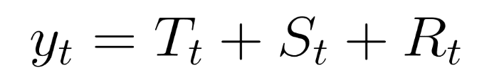
where yt is the data, Tt is the trend-cycle component, St is the seasonal component and Rt is the residual component, all defined over the time period t.
An important first step in describing various components of the series is smoothing, although it does not really provide you with a ready-to-use model. In the beginning, we estimated the trend (behavior) component. Such methods as Moving Average, Exponential Smoothing, Chow’s Adaptive Control, Winter’s Linear and Seasonal Exponential Smoothing methods did not provide us with the trend estimation accuracy we expected. The most reliable result was obtained using the Hodrick-Prescott Filter technique.

Fig. 2. The estimated trend
Then, we defined the seasonality from the available data. This component could change over time, so we applied a powerful tool for decomposing the time series – the Loess method. This approach can handle any type of seasonality, and the rate of change can be controlled by a user.

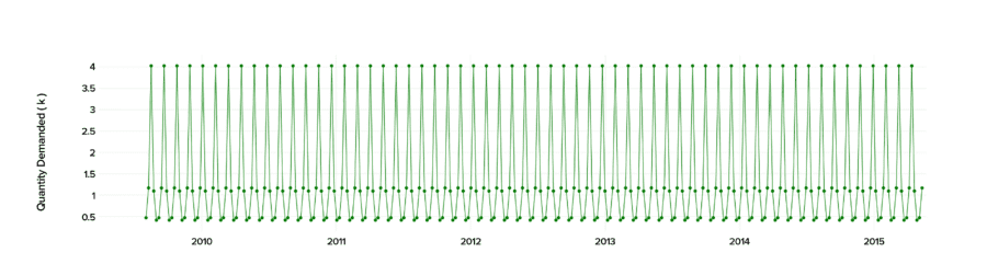
Fig. 3. Multi-seasonality
We obtained a multi-seasonal component with some high and low variances, causing large fluctuations.
After applying Elastic Net Regression and Fourier transformation, we built a forecast for the trend based on the results obtained. The approximation of the trend can be found from the formula below,
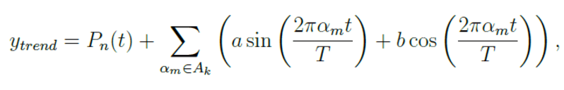
where Pn(t) is a degree polynomial and Ak is a set of indexes, including the first k indexes with highest amplitudes.
Then, we calculated the Fourier coefficients using The Discrete Fourier Transform (DFT).
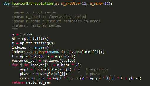
Fig. 4. The example of code of the DFT in Python
The effect of the Fourier terms, used as external regressors in the model, is visualised below.
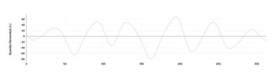
Fig. 5. The visualised effect of Fourier terms
We built the trend prediction using the additive model.

Fig. 6. Trend prediction
When the trend and seasonal components are removed from the model, we can obtain the residuals (the difference between an observed value and its forecast based on other observations) from the remaining part to validate and fit our mathematical model.

Fig. 7. Obtained residuals
You may notice that there are some negative values present, showing that something unusual was happening during that period of time. We aimed to find out the circumstances causing such behaviour, so we came up with an idea to compile the outliers with a simple calendar and discovered that the negative values tightly correlate with such public holidays as Ramadan, Eid Al Fitr and other. Having collected and summarized all the data, we applied Machine Learning methods based on previous data points as entry features and Machine Learning Strategies for Time Series Prediction.
After a few training sessions conducted with ML models, we built a prediction for residuals that can be observed below.

Fig. 8. Prediction for residuals
As a result, we got a final forecasting model that minimizes the mean absolute percentage error (MAPE) to 6% for one particular city and 10% for the entire country in general.
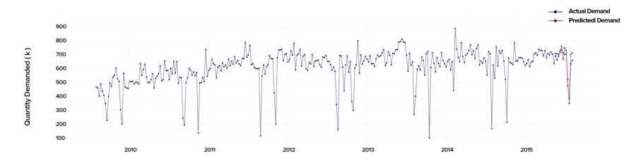
Fig. 9. The forecast at the original scale
A 24-times faster prediction? Yes, it’s possible
When building our model, we attempted not only to use the available information, but also discover the factors which could affect the results. This approach helped us develop the model generating more accurate forecasting results faster than the existing models. For example, to train the developed model to make a prediction for 300 different cities, we need about 15 minutes, while other methods require about 6 hours.
Also, the fact that the deviation between the actual demand and the predicted demand was only 6% resulted in possibilities to resolve mismatches between supply and demand. Now, the customer can more quickly and more easily plan the capacity, minimize future risks and optimize inventory.
What’s next?
Well, the results are quite promising. And there is a long way we can go further in improvement of this model, so it could provide accurate long-term forecasts as well. As for now, the degree of error for long-term predictions is still quite high. Sounds like a challenge? So stay tuned! Some new experiments are coming!
Originally posted here.