
Continued fractions are usually considered as a beautiful, curious mathematical topic, but with applications mostly theoretical and limited to math and number theory. Here we show how it can be used in applied business and economics contexts, leveraging the mathematical theory developed for continued fraction, to model and explain natural phenomena.
The interest in this project started when analyzing sequences such as x(n) = { nq } = nq – INT(nq) where n = 1, 2, and so on, and q is an irrational number in [0, 1] called the seed. The brackets denote the fractional part function. The values x(n) are also in [0, 1] and get arbitrarily close to 0 and 1 infinitely often, and indeed arbitrarily close to any number in [0, 1] infinitely often. I became interested to see what happens when it gets very close to 1, and more precisely, about the distribution of the arrival times t(n) of successive records. I was curious to compare these arrival times with those from truly random numbers, or from real-life time series such as temperature, stock market or gaming/sports data. Such arrival times are known to have an infinite expectation under stable conditions, though their medians always exist: after all, any record could be the final one, never to be surpassed again in the future. This always happens at some point with the sequence x(n), if q is a rational number — thus our focus on irrational seeds: they yield successive records that keep growing over and over, without end, although the gaps between successive records eventually grow very large, in a chaotic, unpredictable way, just like records in traditional time series.
See also my article Distribution of Arrival Times for Extreme Events, here. It turns out that the behavior of the records in the sequence x(n) can be different from those of random numbers, offering a new, broader class of statistical models.
1. Theoretical background (simplified)
In some sense, continued fractions provide the best rational approximations to irrational numbers such as q. The successive approximations, called convergents, converge to q. Let’s look at the sequence of successive records for q = SQRT(2)/2, to see how they are related to the denominators of its convergents in its continued fraction expansion. This is illustrated in the table below.
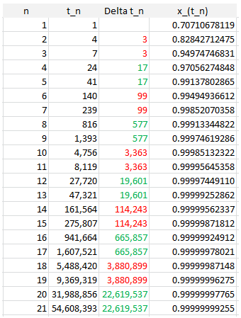 If you do a Google search for (say) “19601 114243”, the first search result is this: A001541 – OEIS. Interestingly, this sequence corresponds to denominators of convergents for SQRT(2)/2. In this case, the arrival times t(n) of the records have an explicit formula:
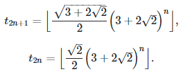
More details are available here. In general, if q is the square root of an integer (not a perfect square) the convergents can be computed explicitly: see here (PDF document). See also here for recurrence relationships. The interesting fact is that t(n), the arrival time of the n-th record, as n grows, is very well approximated by A * B^n (here B^n means B at power n) where A and B are two constants depending on q.
Now let’s turn to q = e = exp(1). The behavior is more chaotic, and pictured in the table below.
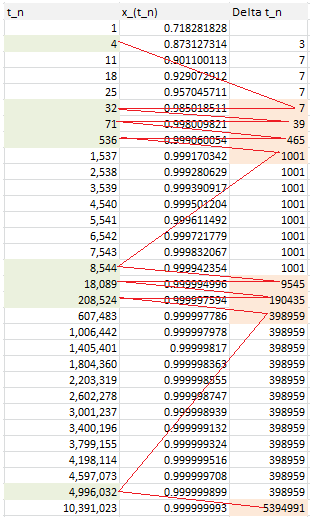
Follow the red path! The first 20 convergents of e are listed below (source: here). Look at the denominator of each convergent to identify the pattern in the red path:
- 8 / 3,
- 11 / 4,
- 19 / 7,
- 87 / 32,
- 106 / 39,
- 193 / 71,
- 1264 / 465,
- 1457 / 536,
- 2721 / 1001,
- 23225 / 8544,
- 25946 / 9545,
- 49171 / 18089,
- 517656 / 190435,
- 566827 / 208524,
- 1084483 / 398959,
- 13580623 / 4996032,
- 14665106 / 5394991,
- 28245729 / 10391023,
- 410105312 / 150869313,
- 438351041 / 161260336
The same pattern applies to all irrational numbers. Indeed, we found an alternate way to compute the convergents, based on the records and their arrival times!
2. Generalization and potential applications to real life problems
We found a connection between records (maxima) of some sequences, and continued fractions. Doing the same thing with minima will complete this analysis. Extreme events in business or economics settings are typically modeled using statistical distributions (Gumbel and so on), which did not live to their expectations in many instances.
The theory outlined here provides an alternative, with each number q serving as a particular model, with its own features distinct from all other numbers. In particular, the numerators and denominators of convergents of q can be used to model the arrival times of extreme events. While the records here are getting closer either to zero or to one, using a logarithm transformation allows you to model phenomena that are not bounded. You can then do some model fitting to find which number q provides the best match with your observations, and use it for predictions.
Note that the sequence x(n) has strong, long-range auto-correlations that are well studied (see appendix B in this book). One could try with the sequence x(n) = { b^n q } instead (b > 1) as it exhibits exponentially fast decaying auto-correlations, also studied in the same book. Even cross-correlations between two sequences have been studied: for instance, if x(n) = { nq } and y(n) = { nq * 12 / 35 }, then the correlation between the two sequences is 1 / (12 * 35). Replace 12 and 35 by any integers that do not share a common divisor, and as long as q is irrational, this result easily generalizes. For a proof, see here. This allows you to model multivariate time series and their cross-dependencies.
Finally, by googling some of the t(n) attached to q = log(3) / log(2) and discussed in the next section, I found that the associated convergents have some applications in music. See here for details.
3. Original applications in music and probabilistic number theory
We focus here on q = log(3) / log(2). The music application is discussed here, and in this section we focus only on the number theory application. The purpose is to prove that the binary digits of SQRT(2) are uniformly distributed, with the proportion of 0 and 1 converging to 50/50 as you look at increasingly longer sequences of successive digits. The use of convergents here helps only with a very specific, narrow part of the proof, but a critical one (assuming a complete proof is ever found – to this day it is still a mystery.)
Let’s look at the sequence z(n) = 2^(-x(n)). with x(n) = { nq } as usual. Since x(n) is equidistributed modulo one, it is uniformly distributed on [0, 1]. Thus the distribution of z(n) is that of 2^(-X) where X is uniformly distributed on [0, 1]. and its median is thus SQRT(2)/2. If n is odd, the empirical median of (z(1), z(2), …, z(n)) is the middle value when these values are sorted, so it is also one of these values. The empirical median converges to the theoretical median SQRT(2)/2. Also, each z(n) is a rational number: the length of its period in base 2 is equal to 2 * 3^(n-1). In addition, the proportion of 0 and 1 in the binary expansion of z(n) and thus in the empirical median regardless of n, is always exactly 50/50. While this is true for all n, it does not mean that this fact remains true for the limit of any converging infinite sub-sequence of z(n) values. Take the sub-sequence z(t(n)) with t(n) the arrival time of the records of x(n). That sub-sequence converges to 1/2. This is a counter-example, and the link to the continued fractions discussed earlier. Sub-sequences having that defect can and sometimes do converge to a non-normal number as in our example, and they must be excluded by carefully removing an infinite number of x(n) without impacting the median. That’s where these records and associated continued fractions become handy.
3.1. Fixing the issue
You don’t need to take all the x(n)’s into consideration. You can choose a sub-sequence x(h(n)) where h(n) is a strictly increasing sequence of integers with { h(n)q } equidistributed mod 1. For instance, h(n) being the n-th prime number, or h(n) being an integer power of n (see here and corollary 6 in this tutorial). Then the distribution of the sequence z(n), including its limiting median SQRT(2)/2, is preserved. Hopefully, one can find such a sequence h(n) that avoids the issues discussed in the previous paragraph.
Another way to remove infinitely many x(n) while preserving the median is by removing selected x(n)’s in a uniform way. If the thinning process used to select which x(n) to keep is uniform over all the original x(n)’s, then the limiting statistical distribution will be unchanged. Or if each time you remove an x(n) smaller than SQRT(2)/2, you also remove one larger than SQRT(2)/2 and conversely, then the limiting median will be unchanged.
Exercise (important): Let q = log(3) / log(2) and w(n) = | x(n) – 1/2 | = | { nq } – 1/2 |. Find the arrival times of the first records for w(n), focusing on minima rather than maxima this time. Let t(n) denotes the arrival time of the n-th record. The sequence D(n) = t(n) – t(n-1) is a subsequence of the one listed here . Again, we have a similar connection with music theory and the convergents of q. Also, D(6) = D(7) = … = D(17) = 665, and D(20) = D(21) = … = D(47) = 190537. Most importantly, the sequence of rational numbers z(t(n)) = 2^(-x(t(n))) converges to SQRT(2)/2. Look at the first n binary digits of z(t(n)), and compute the proportion of zeros and ones. Now do the same analysis with w(n) = | x(n) – 1/e |. The same D(n) show up (almost), in particular D(9) = D(10) = … = D(17) = 665 and D(19) = D(20) = … = D(38) = 190537. However D(8) = 4296 is unusually large. See here for more.
3.2. A deeper result
The table for t(n) for q = (log 3) / (log 2) can be found here. Even though no one has ever fully proved that SQRT(2) has its binary digits uniformly distributed, a much deeper result is “known” (but of course, also unproved) and published here for the first time:
The proportion q(n) of binary digits of SQRT(2) (or any other normal number for that matter, say Pi or log 2), among the first n digits, that are equal to one, satisfies
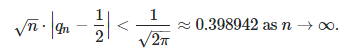
See here for details. In short, this is a consequence of a refined version of the Berry-Esseen theorem, itself a second-order refinement of the central limit theorem. It is true if the digits in question were distributed uniformly and independently with a Bernouilli distribution of parameter 1/2, as they appear to be. Empirical evidence seems to confirm this conjecture: the chart below shows the first 1,000,000 values of SQRT(n) * |q(n) – 1/2|.
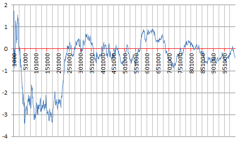
The time series in the above chart looks like a Brownian motion. However, it is not, because it is bounded. In a true Brownian motion, the variance grows infinitely over time. It would be very interesting to study the distribution of the records as well as their values, in that time series. Currently, other than conjectures, very little is known for sure about the distribution of the binary digits of SQRT(2). Some weak results have been proved though, see for instance here. According to this article, the best result proven so far is that q(n) is larger than SQRT(2n) / n for n large enough, which is indeed a very weak result.
To not miss our future articles (more on this topic coming soon), subscribe to our newsletter, here.