
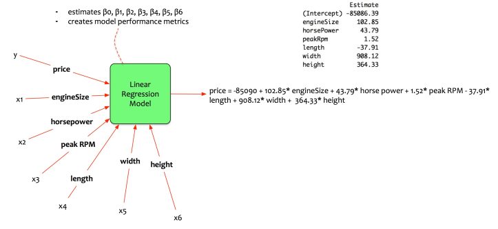
In the last article of this series, we had discussed multivariate linear regression model. Fernando creates a model that estimates the price of the car based on five input parameters.
Fernando indeed has a better model. Yet, he wanted to select the best set of variables for input.
This article will elaborate on model selection methods
Concept
The idea of model selection method is intuitive. It answers the following question:
How to select the right input variables for an optimal model?
How is an optimal model defined?
An Optimal model is the model that fits the data with best values for the evaluation metrics.
There can be a lot of evaluation metrics. The adjusted r-squared is the chosen evaluation metrics for multivariate linear regression models.
There are three methods for selecting the best set of variables. They are:
- Best Subset
- Forward Stepwise
- Backward Stepwise
Let us dive into the inner workings of these methods.
Best Subset
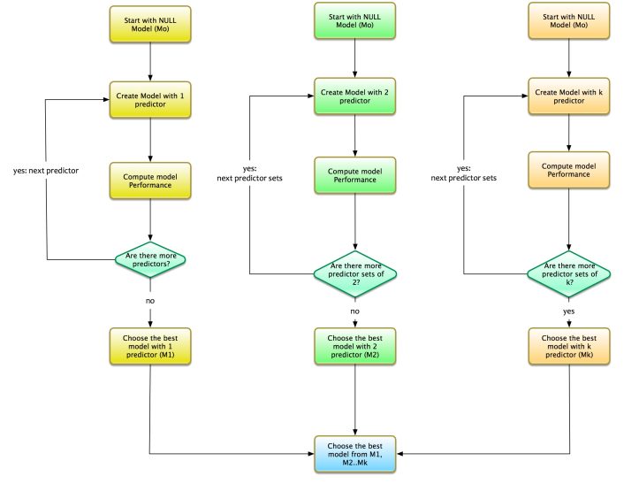
Let us say that we have k variables. The process for best subset method is as follows:
- Start with the NULL model i.e. model with no predictors. Let us call this model as M0.
- Find the optimal model with 1 variable. This means that the model is a simple regressor with only one independent variable. Let us call this model as M1.
- Find the optimal model with 2 variables. This means that the model is a regressor with only two independent variables. Let us call this model as M2.
- Find the optimal model with 3 variables. This means that the model is a regressor with only three independent variables. Let us call this model as M3.
- And so on…We get the drill. Repeat this process. Test all the combination of predictors for the optimal model.
For k variables we need to choose the optimal model from the following set of models:
- M1: The optimal model with 1 predictor.
- M2: The optimal model with 2 predictors.
- M3: The optimal model with 3 predictors.
- Mk: The optimal model with k predictors.
Choose The best model among M1…Mk i.e. the model that has the best fit
The best subset is an elaborate process. It combs through the entire list of predictors. It chooses the best possible combination. However, It has its own challenges.
Best subset creates a model for each predictor and its combination. This implies that we are creating models for each combination of variables. The number of models can be a very large number.
If there are 2 variables then there are 4 possible models. If there are 3 variables then there are 8 possible models. In general, if there are p variables then there are 2^p possible models. That is quite many models to choose from. Imagine that there are 100 variables (quite common). Imagine that there are 100 variables (quite common). There will be 2^100possible models. A mind boggling number.
In Fernando’s case, with only 5 variables, he will have to create and choose from 2^5models i.e. 32 different models.
Forward Stepwise
Although best subset is exhaustive, it requires a lot of computation capabilities. It can be very time-consuming. Forward stepwise tries to ease that pain.
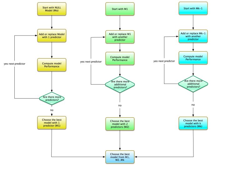
Let us say that we have k variables. The process for the forward stepwise is as follows:
- Start with the NULL model i.e. model with no predictors. We call this M0. Add predictor to model. One at a time.
- Find the optimal model with 1 variable. This means that the model is a simple regressor with only one independent variable. We call this model as M1.
- Add one more variable to M1. Find the optimal model with 2 variables. Note that the additional variable is added to M1. We call this model as M2.
- Add one more variable to M2. Find the optimal model with 3 variables. Note that the additional variable is added to M2. We call this model as M3.
- And so on..We get the drill. Repeat this process until Mk i.e. model with only k variable.
For k variables we need to choose the optimal model from the following set of models:
- M1: The optimal model with 1 predictor.
- M2: The optimal model with 2 predictors. This model is M1 + an extra variable.
- M3: The optimal model with 3 predictors. This model is M2 + an extra variable.
- Mk: The optimal model with k predictors. This model is Mk-1 + an extra variable.
Again, the best model among M1…Mk is chosen i.e. the model that has the best fit
The forward stepwise selection creates fewer models as compared to best subset method. If there are p variables then there will be approximately p(p+1)/2 + 1 models to choose from. Much lower than the model selection from best subset method. Imagine that there are 100 variables; the number of models created based on the forward stepwise method is 100 * 101/2 + 1 i.e. 5051 models.
In Fernando’s case, with only 5 variables, he will have to create and choose from 5*6/2 + 1 models i.e. 16 different models.
Backward Stepwise
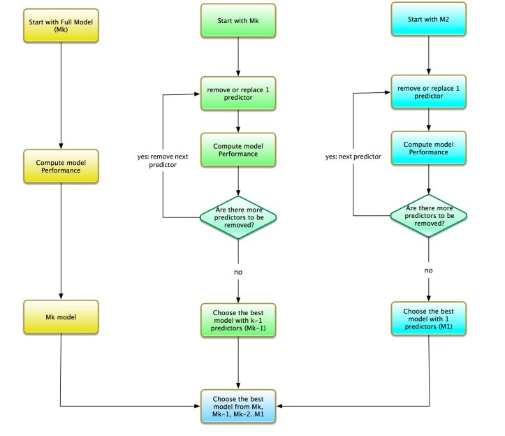
Now that we have understood the forward stepwise process of model selection. Let us discuss the backward stepwise process. It is the reverse of the forward stepwise process. The forward stepwise starts with a model with no variable i.e. NULL model. On the contrast, backward stepwise starts with all the variables. The process for the backward stepwise is as follows:
- Let us say that there are k predictors. Start with a full model i.e. model with all the predictors. We call this model Mk. Remove predictors from the full model. One at a time.
- Find the optimal model with k-1 variable. Remove one variable from Mk. Compute performance of the model for all possible combination. The best model with k-1 variables is chosen. We call this model as Mk-1.
- Find the optimal model with k-2 variable. Remove one variable from Mk-1. Compute performance of the model for all possible combination. The best model with k-2 variables is chosen. We call this model as Mk-2.
- And so on..We get the drill. Repeat this process until M1 i.e. model with only 1 variable.
For k variables we need to choose the optimal model from the following set of models:
- Mk: The optimal model with k predictors.
- Mk-1: The optimal model with k — 1 predictors. This model is Mk — an additional variable.
- Mk-2: The optimal model with k — 2 predictors. This model is Mk — two additional variables.
- M1: The optimal model with 1 predictor.
Model Building
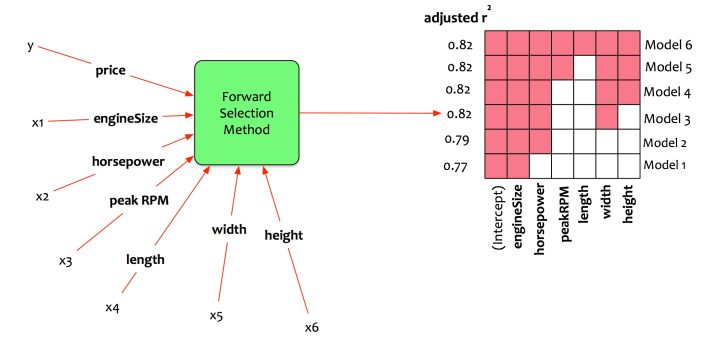
Now that the concepts of model selection are clear, let us get back to Fernando. Recall the previous article of this series. Fernando has six variables engine size, horse power, peak RPM, length, width, and height. He wants to estimate the car price by creating a multivariate regression model. He wants to maintain a balance and choose the best model.
He chooses to apply forward stepwise model selection method. The statistical package computes all the possible models and outputs M1 to M6.
Let us interpret the output.
- Model 1: It should have only one predictor. The best fit model uses only engine size as the predictor. Adjusted R-squared is 0.77.
- Model 2: It should have only two predictors. The best fit model uses only engine size and horsepower as predictors. Adjusted R-squared is 0.79.
- Model 3: It should have only three predictors. The best fit model uses only engine size, horsepower, and width as predictors. Adjusted R-squared is 0.82.
- Model 4: It should have only four predictors. The best fit model uses only engine size, horsepower, width and height as predictors. Adjusted R-squared is 0.82.
- Model 5: It should have only five predictors. The best fit model uses only engine size, horsepower, peak rpm, width and height as predictors. Adjusted R-squared is 0.82.
- Model 6: It should have only six predictors. The best fit model uses only all the six predictors. Adjusted R-squared is 0.82.
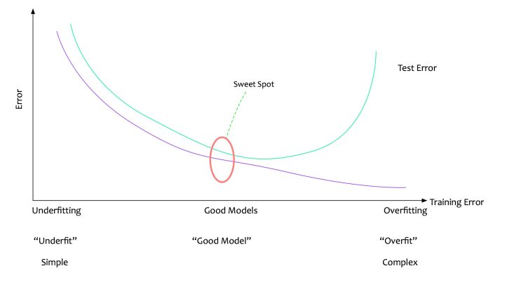
Recall the discussion on creating the simplest yet effective models.
“All models should be made as simple as possible, but no simpler.”
Fernando chooses the simplest model that gives the best performance. In this case, it is Model 3. The model uses engine size, horse power, and width as predictors. The model is able to get an adjusted R-squared of 0.82 i.e. the model can explain 82% of the variations in training data.
The statistical package provides the following coefficients.
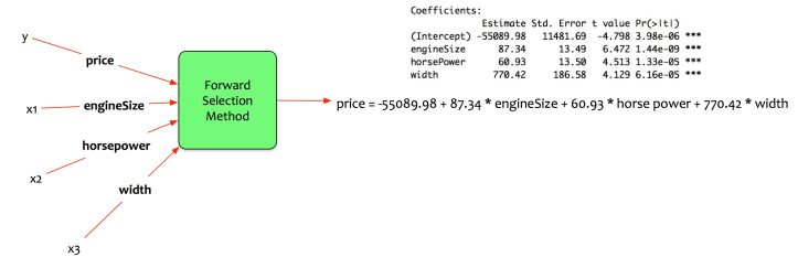
Estimate price as a function of engine size, horse power and width.
price = -55089.98 + 87.34 engineSize + 60.93 horse power + 770.42 width
Model Evaluation
Fernando has chosen the best model. The model will estimate price using engine size, horse power, and width of the car. He wants to evaluate the performance of the model on both training and test data.
Recall, that he had split the data into training and testing sets. Fernando trained the model using the training data. Testing data is unseen data. Fernando evaluates the performance of the model on testing data. That is the real test.
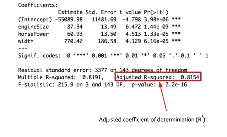
On the training data, the model performs quite well. The adjusted R-squared is 0.815 => the model can explain 81% variation on training data. However, for the model to be acceptable, it also needs to perform well on the testing data.
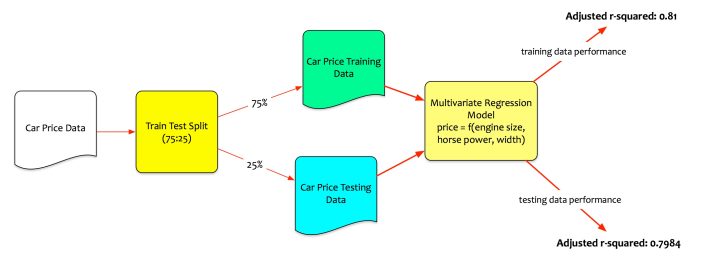
Fernando tests the model performance on test data set. The model computes the adjusted R-squared as 0.7984 on testing data. It means that model can explain 79.84% of variation even on unseen data.
Conclusion
Fernando now has a simple yet effective model that predicts the car price. However, the units of engine size, horse power and width are different. He contemplates.
- How can I estimate the price changes using a common unit of comparison?
- How elastic is the price with respect to engine size, horse power, and width?
The next article of the series is on the way. It will discuss the methods to transform multivariate regression models to compute elasticity.
Originally published at here