
Inference
In a previous blog (The difference between statistics and data science), I discussed the significance of statistical inference. In this section, we expand on these ideas
The goal of statistical inference is to make a statement about something that is not observed within a certain level of uncertainty. Inference is difficult because it is based on a sample i.e. the objective is to understand the population based on the sample. The population is a collection of objects that we want to study/test. For example, if you are studying quality of products from an assembly line for a given day, then the whole production for that day is the population. In the real world, it may be hard to test every product – hence we draw a sample from the population and infer the results based on the sample for the whole population.
In this sense, the statistical model provides an abstract representation of the population and how the elements of the population relate to each other. Parameters are numbers that represent features or associations of the population. We estimate the value of the parameters from the data. A parameter represents a summary description of a fixed characteristic or measure of the target population. It represents the true value that would be obtained as if we had taken a census (instead of a sample). Examples of parameters include Mean (μ), Variance (σ²), Standard Deviation (σ), Proportion (π). These values are individually called a statistic. A Sampling Distribution is a probability distribution of a statistic obtained through a large number of samples drawn from the population. In sampling, the confidence interval provides a more continuous measure of un-certainty. The confidence interval proposes a range of plausible values for an unknown parameter (for example, the mean). In other words, the confidence interval represents a range of values we are fairly sure our true value lies in. For example, for a given sample group, the mean height is 175 cms and if the confidence interval is 95%, then it means, 95% of similar experiments will include the true mean, but 5% will not contain the sample.
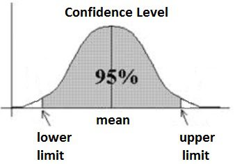
Image source and reference: An introduction to confidence intervals
Hypothesis testing
Having understood sampling and inference, let us now explore hypothesis testing. Hypothesis testing enables us to make claims about the distribution of data or whether one set of results are different from another set of results. Hypothesis testing allows us to interpret or draw conclusions about the population using sample data. In a hypothesis test, we evaluate two mutually exclusive statements about a population to determine which statement is best supported by the sample data. The Null Hypothesis(H0) is a statement of no change and is assumed to be true unless evidence indicates otherwise. The Null hypothesis is the one we want to disprove. The Alternative Hypothesis: (H1 or Ha) is the opposite of the null hypothesis, represents the claim that is being testing. We are trying to collect evidence in favour of the alternative hypothesis. The Probability value (P-Value) represents the probability that the null hypothesis is true based on the current sample or one that is more extreme than the current sample. The Significance Level (α) defines a cut-off p-value for how strongly a sample contradicts the null hypothesis of the experiment. If P-Value < α, then there is sufficient evidence to reject the null hypothesis and accept the alternative hypothesis. If P-Value > α, we fail to reject the null hypothesis.
Central limit theorem
The central limit theorem is at the heart of hypothesis testing. Given a sample where the statistics of the population is unknowable, we need a way to infer statistics across the population. For example, if we want to know the average weight of all the dogs in the world, it is not possible to weigh up each dog and compute the mean. So, we use the central limit theorem and the confidence interval which enables to infer the mean of the population within a certain margin.
So, if we take multiple samples – say the first sample of 40 dogs and compute of the mean for that sample. Again, we take a next sample of say 50 dogs and do the same. We repeat the process by getting a large number of random samples which are independent of each other – then the ‘mean of the means’ of these samples will give the approximate mean of the whole population as per the central limit theorem. Also, the histogram of the means will represent the bell curve as per the central limit theorem. The central limit theorem is significant because this idea applies to an unknown distribution (ex: Binomial or even a completely random distribution) – which means techniques like hypothesis testing can apply to any distribution (not just the normal distribution)
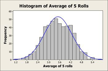
Image source: minitab.