
There is no statistical test that assesses whether a sequence of observations, time series, or residuals in a regression model, exhibits independence or not. Typically, what data scientists do is to look at auto-correlations and see whether they are close enough to zero. If the data follows a Gaussian distribution, then absence of auto-correlations implies independence. Here however, we are dealing with non-Gaussian observations. The setting is similar to testing whether a pseudo-random number generator is random enough, or whether the digits of a number such as π behave in a way that looks random, even though the sequence of digits is deterministic. Batteries of statistical tests are available to address this problem, but there is no one-fit-all solution.
Here we propose a new approach. Likewise, it is not a panacea, but rather a set of additional powerful tools to help test for independence and randomness. The data sets under consideration are specific mathematical sequences, some of which are known to exhibit independence / randomness or not. Thus, it constitutes a good setting to benchmark and compare various statistical tests and see how well they perform. This kind of data is also more natural and looks more real than synthetic data obtained via simulations.
1. Definition of random-like sequences
Since we are dealing with deterministic sequences (xn) indexed by n = 1, 2, and so on, it is worth defining what we mean by independence and random-like. These two elementary concepts are very intuitive, but a formal definition may help. You may skip this section if you have an intuitive understanding of the concepts in question, as the layman does. Independence in this context is sometimes called asymptotic independence, see here. Also, for all the sequences investigated here, xn ∈ [0,1].
1.1. Definition of random-like and independence
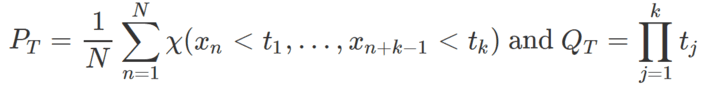
A sequence (xn) with xn ∈ [0,1] is random-like if it satisfies the following property. For any finite index family h1,…, hk and for any t1,…, tk ∈ [0,1], we have
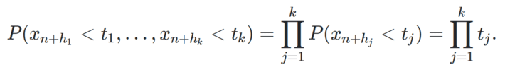
The probabilities are empirical probabilities, that is, based on frequency counts. For instance,
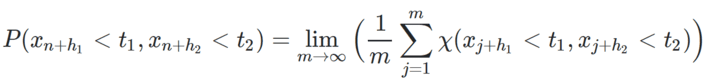
where χ(A) is the indicator function (equal to 1 if the event A is true, and equal to 0 otherwise). Random-like implies independence, but the converse is not true. A sequence is independently distributed if it satisfies the weaker property
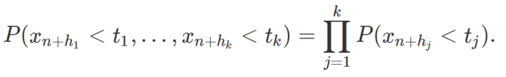
Random-like means that the xn‘s all have the same underlying uniform distribution on [0, 1], and are independently distributed.
1.2. Definition of lag-k autocorrelation
Again, this is just the standard definition of auto-correlations, but applied to infinite deterministic sequences. The lag-k auto-correlation ρk is defined as follows. First define ρk(n) as the empirical correlation between (x1,…, xn) and (xk+1,… ,xk+n). Then ρk is the limit (if it exists) of ρk(n) as n tends to infinity.
1.3. Equidistribution and fractional part denoted as { }
The fractional part of a positive real number x is denoted as { x }. For instance, { 3.141592 } = 0.141592. The sequences investigated here come from number theory. In that context, concepts such as random-like and identically distributed are rarely used. Instead, mathematicians rely on the weaker concept of equidistribution, also called equidistribution modulo 1. Closer to independence is the concept of equidistribution in higher dimensions, for instance if two successive values (xn, xn+1) are equidistributed on [0, 1] x [0, 1].
A sequence can be equidistributed yet exhibits strong auto-correlations. The most famous example is the sequence xn = { αn } where α is a positive irrational number. While equidistributed, it has strong lag-k auto-correlations for every strictly positive integer k, and it is anything but random-like. A sequence that looks perfectly random-like is the digits of π: they can not be distinguished from a realization of a perfect Bernouilli process. Such random-like sequences are very useful in cryptographic applications.
2. Testing well-known sequences
The sequences we are interested in are xn = { α n^p } where { } is the fractional part function (see section 1.3), p > 1 is a real number and α is a positive irrational number. Other sequences are discussed in section 3. It is well known that these sequences are equidistributed. Also, if p = 1, these sequences are highly auto-correlated and thus the terms xn‘s are not independently distributed, much less random-like; the exact theoretical lag-k auto-correlations are known. The question here is what happens if p > 1. It seems that in that case, there is much more randomness. In this section, we explore three statistical tests (including a new one) to assess how random these sequences can be depending on the parameters p and α. The theoretical answer to that question is known, thus this provides a good case study to check how various statistical tests perform to detect randomness, or lack of it.
2.1. The gap test
The gap test (some people may call it run test) proceeds as follows. Let us define the binary digit dn as dn = ⌊2xn⌋. The brackets represent the integer part function. Say dn = 0 and dn+1 = 1 for a specific n. If dn is followed by G successive digits dn+1,…, dn+G all equal to 1 and then dn+G+1 = 0, we have one instance of a gap of length G. Compute the empirical distribution of these gaps. Assuming 50% of the digits are 0 (this is the case in all our examples), then the empirical gap distribution converges to a geometric distribution of parameter 1/2 if the sequence xn is random-like.
This is best illustrated in chapter 4 of my book Applied Stochastic Processes, Chaos Modeling, and Probabilistic Properties of Numeration Systems, available here.
2.2. The collinearity test
Many sequences pass several tests yet fail the collinearity test. This test checks whether there are k constants a1, …, ak with ak not equal to zero, such that xn+k = a1 xn+k-1 + a2 xn+k-2 + … + ak xn takes only on a finite (usually small) number of values. In short, it addresses this question: are k successive values of the sequence xn always lie (exactly, approximately, or asymptotically) in a finite number of hyperplanes of dimension k – 1? This test has been used to determine that some congruential pseudo-random number generators were of very poor quality, see here. It is illustrated in section 3, with k = 2.
Source code and examples for k = 3 can be found here.
2.3. The independence test
This may be a new test: I could not find any reference to it in the literature. It does not test for full independence, but rather for random-like behavior in small dimensions (k = 2, 3, 4). Beyond k = 4, it becomes somewhat unpractical as it requires a number of observations (that is, the number of computed terms in the sequence) growing exponentially fast with k. However, it is a very intuitive test. It proceeds as follows, for a fixed k:
- Let N > 100 be an integer
- Let T be a k-uple (t1,…, tk) with tj ∈ [0,1] for j = 1, …, k.
- Compute the following two quantities, with χ being the indicator function as in section 1.2:
- Repeat this computation for M different k-uples randomly selected in the k-dimensional unit hypercube
Now plot the M vectors (PT, QT), each corresponding to a different k-uple, on a scatterplot. Unless the M points lie very close to the main diagonal on the scatterplot, the sequence xn is not random-like. To see how far away you can be from the main diagonal without violating the random-like assumption, do the same computations for 10 different sequences consisting this time of truly random terms. This will give you a confidence band around the main diagonal, and vectors (PT, QT) lying outside that band, for the original sequence you are interested in, suggests areas where the randomness assumption is violated. This is illustrated in the picture below, originally posted here:
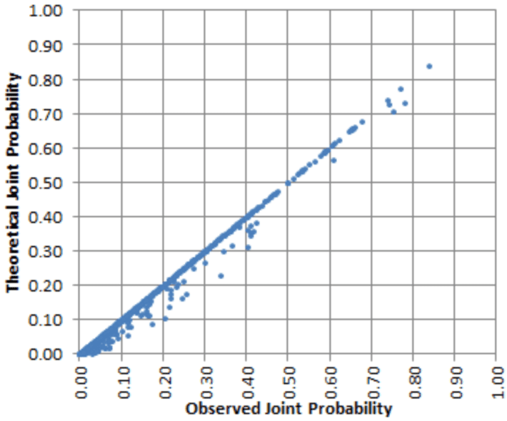
Figure 1
As you can see, there is a strong enough departure from the main diagonal, and the sequence in question (see same reference) is known not to be random-like. The X-axis features PT, and the Y-axis features QT. An example with known random-like behavior, resulting in an almost perfect diagonal, is also featured in the same article. Notice that there are fewer and fewer points as you move towards the upper right corner. The higher k, the more sparse the upper right corner will be. In the above example, k = 3. To address this issue, proceed as follows, stretching the point distribution along the diagonal:
- Let P*T = (- 2 log PT) / k and Q*T = (- 2 log QT) / k. This is a transformation leading to a Gamma(k, 2/k) distribution. See explanations here.
- Let P**T = F(P*T) and Q**T = F(Q*T) where F is the cumulative distribution function of a Gamma(k, 2/k) random variable.
By virtue of the inverse transform sampling theorem, the points (P**T, Q**T) are now uniformly stretched along the main diagonal.
3. Results and generalization
Let’s get back to our sequence xn = { α n^p } with p > 1 and α irrational. Before showing and discussing some charts, I want to discuss a few issues. First, if p is large, machine accuracy will quickly result in erroneous computations for xn. You need to detect when loss of accuracy becomes a critical problem, usually well below n = 1,000 if p = 5. Working with double precision arithmetic will help. Another issue, if p is close to 1, is the fact that randomness does not kick in until n is large enough. You may have to ignore the first few hundreds terms of the sequence in that case. If p = 1, randomness never occurs. Also, we have assumed that the marginal distributions are uniform on [0, 1]. From the theoretical point of view, they indeed are, and it will show if you compute the empirical percentile distribution of xn, even in the presence of strong auto-correlations (the reason why is because of the ergodic nature of the sequences in question, but this topic is beyond the scope of the present article). So it would be a good exercise to use various statistical tools or libraries to assess whether they can confirm the uniform distribution assumption.
3.1. Examples
The exact theoretical value of the lag-k auto-correlation is known for all k if p = 1. See section 5.4 in this article. It is almost never equal to zero, but it turns out that if k = 1, p = 1 and α = (3 + SQRT(3))/6, it is indeed equal to zero. Use a statistical package to see if it can detect this fact, or ask your team to do the test. Also, if p is an integer, show (using statistical techniques) that for some a1, …, ak, we have xn+k = a1 xn+k-1 + a2 xn+k-2 + … + ak xn takes only on a finite number of values as discussed in section 2.2, and thus, the random-like assumption is always violated. In particular, k = 2 if p = 1. This is also true asymptotically if p is not an integer, see here for details. Yet, if p > 1, the auto-correlations are very close to zero, unlike the case p = 1. But are they truly identical to zero? What about the sequence xn = { α^n } with say α = log 3? Is it random-like? Nobody knows. Of course, if α = (1 + SQRT(5))/2, that sequence is anything but random, so it depends on α.
Below are three scatterplots showing the distribution of (xn, xn+1) for a few hundreds value of n, for various α and p, for the sequence xn = { α n^p }. The X-axis represents xn, the Y-axis represents xn+1.
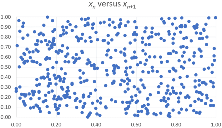
Figure 2: p = SQRT(7), α = 1
Even to the trained naked eye, Figure 2 shows randomness in 2 dimensions. Independence may fail in higher dimensions (k > 2) as the sequence is known not to be random-like. There is no apparent collinearity pattern as discussed in section 2.2, at least for k = 2. Can you run some test to detect lack of randomness in higher dimensions?
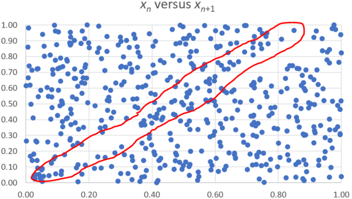
Figure 3: p = 1.4, α = log 2
To the trained naked eye, Figure 3 shows lack of randomness as highlighted in the red band. Can you do a test to confirm this? If the test is inclusive or provide the wrong answer, than the naked eye performs better, in this case, than statistical software.
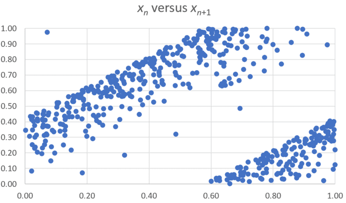
Figure 4: p = 1.1, α = log 2
Here (Figure 4) any statistical software and any human being, even the layman, can identify lack of randomness in more than one way. As p gets closer and closer to 1, lack of randomness is obvious, and the collinearity issue discussed in section 1.2, even if fuzzy, becomes more apparent even in two dimensions.
3.2. Independence between two sequences
It is known that if α and β are irrational numbers linearly independent over the set of rational numbers, then the sequences { αn } and { βn } are not correlated, even though each one taken separately is heavily auto-correlated. A sketch proof of this result can be found in the Appendix of this article. But are they really independent? Test, using statistical software, the absence of correlation if α = log 2 and β = log 3. How would you do to test independence? The methodology presented in section 2.3 can be adapted and used to answer this question empirically (although not theoretically).
About the author: Vincent Granville is a data science pioneer, mathematician, book author (Wiley), patent owner, former post-doc at Cambridge University, former VC-funded executive, with 20+ years of corporate experience including CNET, NBC, Visa, Wells Fargo, Microsoft, eBay. Vincent also founded and co-founded a few start-ups, including one with a successful exit (Data Science Central acquired by Tech Target). You can access Vincent’s articles and books, here.