
KernelML – Hierarchical Density Factorization
Goals
- Approximate any empirical distribution
- Build a parameterized density estimator
- Outlier detection and dataset noise reduction
My Approach
This solution I came up with was incorporated into a python package, KernelML. The example code can be found here.
My solution uses the following:
- Particle Swarm\Genetic Optimizer
- Multi-Agent Approximation using IID Kernels
- Reinforcement Learning
Particle Swarm\Genetic Optimizer
Most kernels have hyper-parameters that control the mean and variation of the distribution. While these parameters are potentially differentiable, I decided against using a gradient-based method. The gradients for the variance parameters can potentially vanish, and constraining the variance makes the parameters non-differentiable. It makes sense to use a mixed integer or particle swarm strategy to optimize the kernels’ hyper-parameters. I decided to use a uniform distribution kernel because of its robustness to outliers in higher dimensions.
Over the past year, I’ve independently developed an optimization algorithm to solve non-linear, constrained optimization problems. It is by no means perfect, but building it from scratch allowed me to 1) make modifications based on the task 2) better understand the problem I was trying to solve.
Multi-Agent Approximation using IID Kernels
My initial approach used a multi-agent strategy to simultaneously fit any multi-variate distribution. The agents, in this case, the kernels, were independent and identically distributed (IID). I made an algorithm, called density factorization, to fit an arbitrary number of agents to a distribution. The optimization approach and details can be found here. The video below shows a frame-by-frame example for how the solution might look over the optimization procedure.
This algorithm seemed to perform well on non-sparse, continuous distributions. One problem was that the algorithm used IID kernels which is an issue when modeling skewed data. Every kernel has the same 1/K weight, where K is the number of kernels. In theory, hundreds of kernels could be optimized at once, but this solution lacked efficiency and granularity.
Reinforcement Learning
I decided to use a hierarchical, reinforcement style approach to fitting the empirical multi-variate distribution. The initial reward, R_0, was the empirical distribution, and the discounted reward, R_1, represented the data points not captured by the initial multi-agent algorithm at R_0. Equation (1) shows the update process for the reward.

Where p is the percentage of unassigned data points, R is the empirical distribution at step t, U is the empirical distribution for the unassigned data points, and lambda is the discount factor. The reward update is the multiplication of p and lambda.
This works because, by definition, the space between data points increases as the density decreases. As data points in under-populated regions are clustered, the cluster sizes will increase to capture new data points. The reward update is less than the percentage of unassigned data point which allows the denser regions to be represented multiple times before moving to the less dense regions.
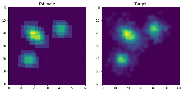
The algorithm uses pre-computed rasters to approximate the empirical density which means that the computational complexity depends on the number of dimensions, not the data points. The example below shows how the estimated and empirical distribution might look for the 2-D case.
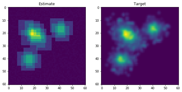
After fitting the initial density factorization algorithm, the reward is updated by some discount factor to improve the reward for the data points that have not been captured. The plot below shows how the empirical distribution might look after a few updates.
The samples in each cluster must be greater than the minimum-leaf-sample parameter. This parameter prevents clusters from accidentally modeling outliers by chance. This is mostly an issue in higher dimensional space due to the curse of dimensionality. If a cluster does not meet this constraint, it is pruned from the cluster solution. This process continues until 1) a new cluster solution does not capture new data points or 2) >99% of the data points have been captured (this threshold is also adjustable).
Example
As the input space increases in dimensionality, the Euclidean space between data points increases. For example, for an input space that contains uniform random variables, the space between space points increases by a factor of sqrt(D), where D is the number of dimensions.
To create a presentable example, the curse of dimensionality will be simulated in 2-D. This can be achieved by creating an under-sampled (sparse) training dataset and an over-sampled validation dataset. Two of the clusters were moved closer together to make cluster separation more difficult.
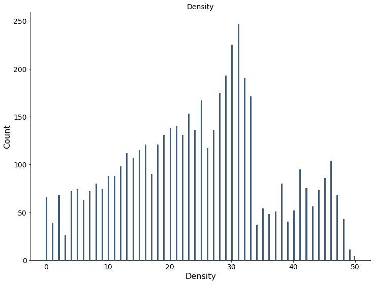
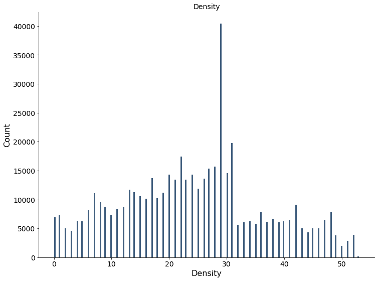
The density can be estimated by counting the number of clusters assigned to a data point. The solution is parameterized so it can be applied to the validation dataset after training. The plot below shows the histogram of the density estimate after running the model on the training dataset.
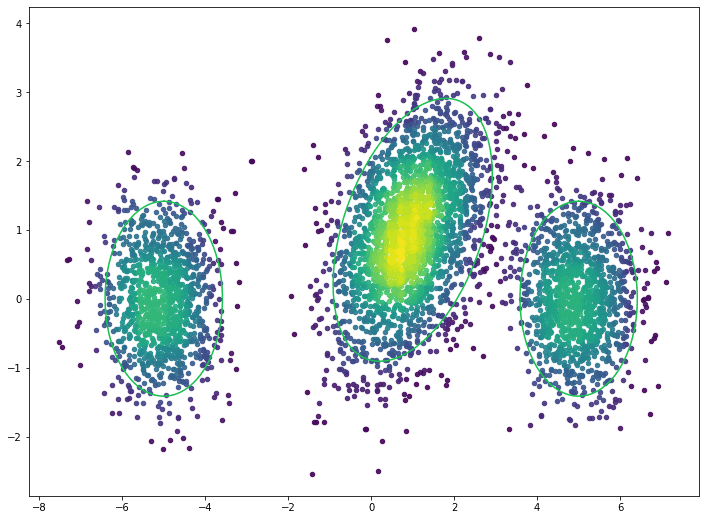
The density can be used to visualize the denser areas of the data. The green rings show the true distributions’ two standard deviation threshold. The plot below visualizes the density for the training dataset.
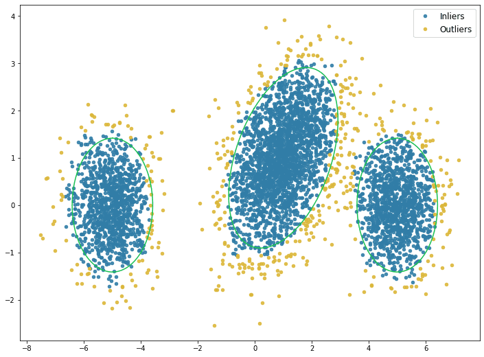
Outliers can be defined by a percentile, i.e. 5th, 10th, etc., of the density estimate. The plot below shows the outliers defined by the 10th percentile. The green rings show the true distributions’ two standard deviation threshold
The plot below shows the histogram of the density estimate for the validation dataset.
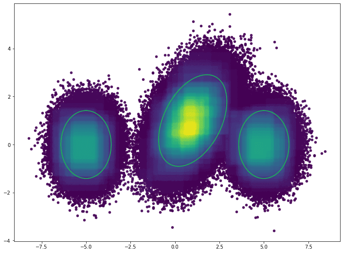
The plot below visualizes the density for the validation dataset. The green rings show the true distributions’ two standard deviation threshold
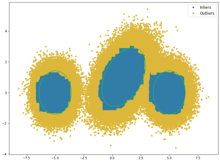
The outliers, defined by the 10th percentile, are visualized below. The green rings show the true distributions’ two standard deviation threshold
Conclusion
This particular use case was focused on outlier detection. However, the algorithm also provided cluster assignments and density estimates for each data point. Other outlier detection methods, i.e., local outlier factor (LOF), can produce similar results in terms of outliers detection. Local outlier factor is dependent on the number of nearest neighbors and the contamination parameter. While it is easy to tune LOF’s parameter in 2-D, it is not so easy in multiple dimensions. Hierarchical density factorization provides a robust method to fit multi-variate distributions without the need for extensive hyper-parameter tuning. While the algorithm does not depend on the number of data points, it is still a relatively slow algorithm. Many improvements can be made to improve the efficiency and speed. The example notebook includes a comparison to LOF and a multivariate example using the Pokemon dataset.
Originally posted here.