

Understanding what a model doesn’t know is important both from the practitioner’s perspective and for the end users of many different machine learning applications. In our previous blog post we discussed the different types of uncertainty. We explained how we can use it to interpret and debug our models.
In this post we’ll discuss different ways to obtain uncertainty in Deep Neural Networks. Let’s start by looking at neural networks from a Bayesian perspective.
Bayesian learning 101
Bayesian statistics allow us to draw conclusions based on both evidence (data) and our prior knowledge about the world. This is often contrasted with frequentist statistics which only consider evidence. The prior knowledge captures our belief on which model generated the data, or what the weights of that model are. We can represent this belief using a prior distribution p(w) over the model’s weights.
As we collect more data we update the prior distribution and turn in into a posterior distribution using Bayes’ law, in a process called Bayesian updating:
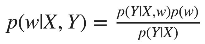
This equation introduces another key player in Bayesian learning — the likelihood, defined as p(y|x,w). This term represents how likely the data is, given the model’s weights w.
Neural networks from a Bayesian perspective
A neural network’s goal is to estimate the likelihood p(y|x,w). This is true even when you’re not explicitly doing that, e.g. when you minimize MSE.
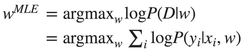
To find the best model weights we can use Maximum Likelihood Estimation (MLE):
Alternatively, we can use our prior knowledge, represented as a prior distribution over the weights, and maximize the posterior distribution. This approach is called Maximum Aposteriori Estimation (MAP):
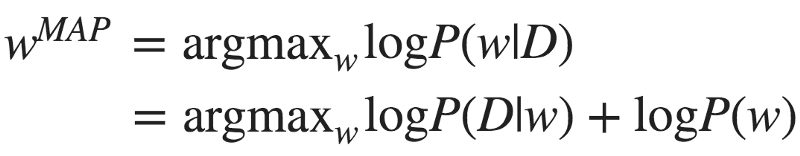
The term logP(w), which represents our prior, acts as a regularization term. Choosing a Gaussian distribution with mean 0 as the prior, you’ll get the mathematical equivalence of L2 regularization.
Now that we start thinking about neural networks as probabilistic creatures, we can let the fun begin. For start, who says we have to output one set of weights at the end of the training process? What if instead of learning the model’s weights, we learn a distribution over the weights? This will allow us to estimate uncertainty over the weights. So how do we do that?
Once you go Bayesian, you never go back
We start again with a prior distribution over the weights and aim at finding their posterior distribution. This time, instead of optimizing the network’s weights directly we’ll average over all possible weights (referred to as marginalization).
At inference, instead of taking the single set of weights that maximized the posterior distribution (or the likelihood, if we’re working with MLE), we consider all possible weights, weighted by their probability. This is achieved using an integral:

x is a data point for which we want to infer y, and X,Y are training data. The first term p(y|x,w) is our good old likelihood, and the second term p(w|X,Y) is the posterior probability of the model’s weights given the data.
We can think about it as an ensemble of models weighted by the probability of each model. Indeed this is equivalent to an ensemble of infinite number of neural networks, with the same architecture but with different weights.
Are we there yet?
Ay, There’s the rub! Turns out that this integral is intractable in most cases. This is because the posterior probability cannot be evaluated analytically.
This problem is not unique to Bayesian Neural Networks. You would run into this problem in many cases of Bayesian learning, and many methods to overcome this have been developed over the years. We can divide these methods into two families: variational inference and sampling methods.
Monte Carlo sampling
We have a problem. The posterior distribution is intractable. What if instead of computing the integral over the true distribution we’ll approximate it with the average of samples drawn from it? One way to do that is the Markov Chain Monte Carlo — you construct a markov chain with the desired distribution as its equilibrium distribution.
Variational Inference
Another solution is to approximate the true intractable distribution with a different distribution from a tractable family. To measure the similarity of the two distribution we can use KL divergence:
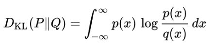
Let q be a variational distribution parameterized by θ. We want to find the value of θ that minimizes the KL divergence:

Look at what we’ve got: the first term is the KL divergence between the variational distribution and the prior distribution. The second term is the likelihood with regards to qθ. So we’re looking for qθ that explains the data best, but on the other hand is as close as possible to the prior distribution. This is just another way to introduce regularization into neural networks!
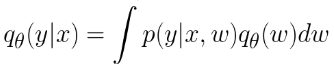
Now that we have qθ we can use it to make predictions:
The above formulation comes from a work by DeepMind in 2015. Similar ideas were presented by graves in 2011 and go back to Hinton and van Campin 1993. The keynote in NIPS Bayesian Deep Learning workshop had a very nice overview of how these ideas evolved over the years.
OK, but what if we don’t want to train a model from scratch? What if we have a trained model that we want to get uncertainty estimation from? Can we do that?
It turns out that if we use dropout during training, we actually can.

Professional data scientists contemplating the uncertainty of their model — an illustration
Dropout as a mean for uncertainty
Dropout is a well used practice as a regularizer. In training time, you randomly sample nodes and drop them out, that is — set their output to 0. The motivation? You don’t want to over rely on specific nodes, which might imply overfitting.
In 2016, Gal and Ghahramani showed that if you apply dropout at inference time as well, you can easily get an uncertainty estimator:
- Infer y|x multiple times, each time sample a different set of nodes to drop out.
- Average the predictions to get the final prediction E(y|x).
- Calculate the sample variance of the predictions.
That’s it! You got an estimate of the variance! The intuition behind this approach is that the training process can be thought of as training 2^m different models simultaneously — where m is the number of nodes in the network: each subset of nodes that is not dropped out defines a new model. All models share the weights of the nodes they don’t drop out. At every batch, a randomly sampled set of these models is trained.
After training, you have in your hands an ensemble of models. If you use this ensemble at inference time as described above, you get the ensemble’s uncertainty.
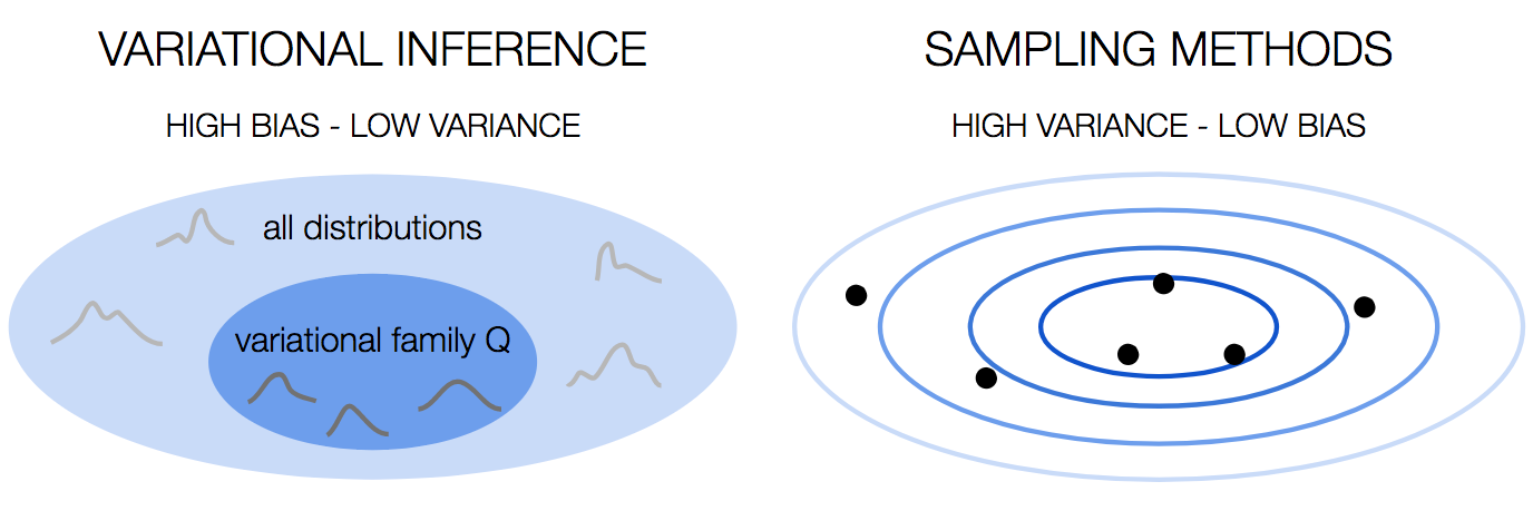
Sampling methods vs Variational Inference
In terms of the bias-variance tradeoff, variational inference has high bias because we choose the distributions family. This is a strong assumption that we’re making, and as any strong assumption, it introduces bias. However, it’s stable, with low variance.
Sampling methods on the other hand have low bias, because we don’t make assumptions about the distribution. This comes at the price of high variance, since the result is dependent on the samples we draw.
Final thoughts
Being able to estimate the model uncertainty is a hot topic. It’s important to be aware of it in high risk applications such as medical assistants and self-driving cars. It’s also a valuable tool to understand which data could benefit the model, so we can go and get it.
In this post we covered some of the approaches to get model uncertainty estimations. There are many more methods out there, so if you feel highly uncertain about it, go ahead and look for more data 🙂
In the next post we’ll show you how to use uncertainty in recommender systems, and specifically — how to tackle the exploration-exploitation challenge. Stay tuned.
This is the second post of a series related to a paper we’re presenting in a workshop in this year KDD conference: deep density networks and uncertainty in recommender systems.
The first post can be found here.
This is a joint post with Inbar Naor. Originally published at engineering.taboola.com