
Principal Component Analysis (PCA) is a technique used to find the core components that underlie different variables. It comes in very useful whenever doubts arise about the true origin of three or more variables. There are two main methods for performing a PCA: naive or less naive. In the naive method, you first check some conditions in your data which will determine the essentials of the analysis. In the less-naive method, you set the those yourself, based on whatever prior information or purposes you had. I will tackle the naive method, mainly by following the guidelines in Field, Miles, and Field (2012), with updated code where necessary.
The ‘naive’ approach is characterized by a first stage that checks whether the PCA should actually be performed with your current variables, or if some should be removed. The variables that are accepted are taken to a second stage which identifies the number of principal components that seem to underlie your set of variables. I ascribe these to the ‘naive’ or formal approach because either or both could potentially be skipped in exceptional circumstances, where the purpose is not scientific, or where enough information exists in advance.
STAGE 1. Determine whether PCA is appropriate at all, considering the variables
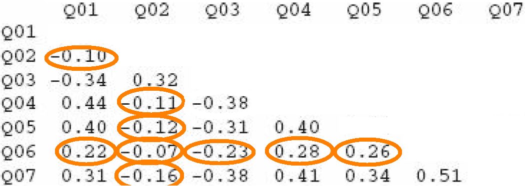
- Variables should be inter-correlated enough but not too much. Field et al. (2012) provide some thresholds, suggesting that no variable should have many correlations below .30, or any correlation at all above .90. Thus, in the example here, variable Q06 should probably be excluded from the PCA.
- Bartlett’s test, on the nature of the intercorrelations, should be significant. Significance suggests that the variables are not an ‘identity matrix’ in which correlations are a sampling error.
- KMO (Kaiser-Meyer-Olkin), a measure of sampling adequacy based on common variance (so similar purpose as Bartlett’s). As Field et al. review, ‘values between .5 and .7 are mediocre, values between .7 and .8 are good, values between .8 and .9 are great and values above .9 are superb’ (p. 761). There’s a general score as well as one per variable. The general one will often be good, whereas the individual scores may more likely fail. Any variable with a score below .5 should probably be removed, and the test should be run again.
- Determinant: A formula about multicollinearity. The result should preferably fall below .00001.
Note that some of these tests are run on the dataframe and others on a correlation matrix of the data, as distinguished below.
# Necessary libraries
library(ltm)
library(lattice)
library(psych)
library(car)
library(pastecs)
library(scales)
library(ggplot2)
library(arules)
library(plyr)
library(Rmisc)
library(GPArotation)
library(gdata)
library(MASS)
library(qpcR)
library(dplyr)
library(gtools)
library(Hmisc)# Select only variables of interest for the PCA
dataset = mydata[, c(‘select_var1′,’select_var1′,’select_var2’,
‘select_var3′,’select_var4′,’select_var5′,’select_var6′,’select_var7’)]# Create matrix: some tests will require it
data_matrix = cor(dataset, use = ‘complete.obs’)
# See intercorrelations
round(data_matrix, 2)# Bartlett’s
cortest.bartlett(dataset)# KMO (Kaiser-Meyer-Olkin)
KMO(data_matrix)# Determinant
det(data_matrix)
STAGE 2. Identify number of components (aka factors)
In this stage, principal components (formally called ‘factors’ at this stage) are identified among the set of variables.
- The identification is done through a basic, ‘unrotated’ PCA. The number of components set a priori must equal the number of variables that are being tested.
# Start off with unrotated PCA
pc1 = psych::principal(dataset, nfactors = length(dataset), rotate="none")
 pc1
Below, an example result:
## Principal Components Analysis
## Call: psych::principal(r = eng_prop, nfactors = 3, rotate = “none”)
## Standardized loadings (pattern matrix) based upon correlation matrix
## PC1 PC2 PC3 h2 u2 com
## Aud_eng -0.89 0.13 0.44 1 -2.2e-16 1.5
## Hap_eng 0.64 0.75 0.15 1 1.1e-16 2.0
## Vis_eng 0.81 -0.46 0.36 1 -4.4e-16 2.0
##
## PC1 PC2 PC3
## SS loadings 1.87 0.79 0.34
## Proportion Var 0.62 0.26 0.11
## Cumulative Var 0.62 0.89 1.00
## Proportion Explained 0.62 0.26 0.11
## Cumulative Proportion 0.62 0.89 1.00
##
## Mean item complexity = 1.9
## Test of the hypothesis that 3 components are sufficient.
##
## The root mean square of the residuals (RMSR) is 0
## with the empirical chi square 0 with prob < NA
##
## Fit based upon off diagonal values = 1
Among the columns, there are first the correlations between variables and components, followed by a column (h2) with the ‘communalities‘. If less factors than variables had been selected, communality values would be below 1. Then there is the uniqueness column (u2): uniqueness is equal to 1 minus the communality. Next is ‘com’, which reflects the complexity with which a variable relates to the principal components. Those components are precisely found below. The first row contains the sums of squared loadings, or eigenvalues, namely, the total variance explained by each linear component. This value corresponds to the number of units explained out of all possible factors (which were three in the above example). The rows below all cut from the same cloth. Proportion var = variance explained over a total of 1. This is the result of dividing the eigenvalue by the number of components. Multiply by 100 and you get the percentage of total variance explained, which becomes useful. In the example, 99% of the variance has been explained. Aside from the meddling maths, we should actually expect 100% there because the number of factors equaled the number of variables. Cumulative var: variance added consecutively up to the last component. Proportion explained: variance explained over what has actually been explained (only when variables = factors is this the same as Proportion var). Cumulative proportion: the actually explained variance added consecutively up to the last component.
Two sources will determine the number of components to select for the next stage:
- Kaiser’s criterion: components with SS loadings > 1. In our example, only PC1.
A more lenient alternative is Joliffe’s criterion, SS loadings > .7.
- Scree plot: the number of points after point of inflexion. For this plot, call:
plot(pc1$values, type = 'b')
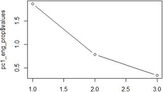
Imagine a straight line from the first point on the right. Once this line bends considerably, count the points after the bend and up to the last point on the left. The number of points is the number of components to select. The example here is probably the most complicated (two components were finally chosen), but normally it’s not difficult.
Based on both criteria, go ahead and select the definitive number of components.
STAGE 3. Run definitive PCA
Run a very similar command as you did before, but now with a more advanced method. The first PCA, a heuristic one, worked essentially on the inter-correlations. The definitive PCA, in contrast, will implement a prior shuffling known as ‘rotation’, to ensure that the result is robust enough (just like cards are shuffled). Explained variance is captured better this way. The go-to rotation method is the orthogonal, or ‘varimax’ (though others may be considered too).
# Now with varimax rotation, Kaiser-normalized by default:
pc2 = psych::principal(dataset, nfactors=2, rotate = “varimax”,
scores = TRUE)
pc2
pc2$loadings# Healthcheck
pc2$residual
pc2$fit
pc2$communality
We would want:
- Less than half of residuals with absolute values > 0.05
- Model fit > .9
- All communalities > .7
If any of this fails, consider changing the number of factors. Next, the rotated components that have been ‘extracted’ from the core of the set of variables can be added to the dataset. This would enable the use of these components as new variables that might prove powerful and useful
dataset <- cbind(dataset, pc2$scores)
summary(dataset$RC1, dataset$RC2)
STAGE 4. Determine ascription of each variable to components
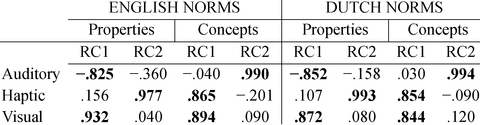
Check the main summary by just calling pc2, and see how each variable correlates with the rotated components. This is essential because it reveals how variables load on each component, or in other words, to which component a variable belongs. For instance, the table shown here belongs to a study about meaning of words. These results suggest that the visual and haptic modalities of words are quite related, whereas the auditory modality is relatively unique. When the analysis works out well, a cut-off point of r = .8 may be applied for considering a variable as part of a component.
STAGE 5. Enjoy the plot
The plot is perhaps the coolest part about PCA. It really makes an awesome illustration of the power of data analysis.
ggplot(dataset,
aes(RC1, RC2, label = as.character(main_eng))) +
aes (x = RC1, y = RC2, by = main_eng) + stat_density2d(color = “gray87”)+
geom_text(size = 7) +
ggtitle (‘English properties’) +
theme_bw() +
theme(
plot.background = element_blank()
,panel.grid.major = element_blank()
,panel.grid.minor = element_blank()
,panel.border = element_blank()
) +
theme(axis.line = element_line(color = ‘black’)) +
theme(axis.title.x = element_text(colour = ‘black’, size = 23,
margin=margin(15,15,15,15)),
axis.title.y = element_text(colour = ‘black’, size = 23,
margin=margin(15,15,15,15)),
axis.text.x = element_text(size=16),
axis.text.y = element_text(size=16)) +
labs(x = “”, y = “Varimax-rotated Principal Component 2”) +
theme(plot.title = element_text(hjust = 0.5, size = 32, face = “bold”,
margin=margin(15,15,15,15)))
Below is an example combining PCA plots with code similar to the above. These plots illustrate something further with regard to the relationships among modalities. In property words, the different modalities spread out more clearly than they do in concept words. This makes sense because in language, properties define concepts .
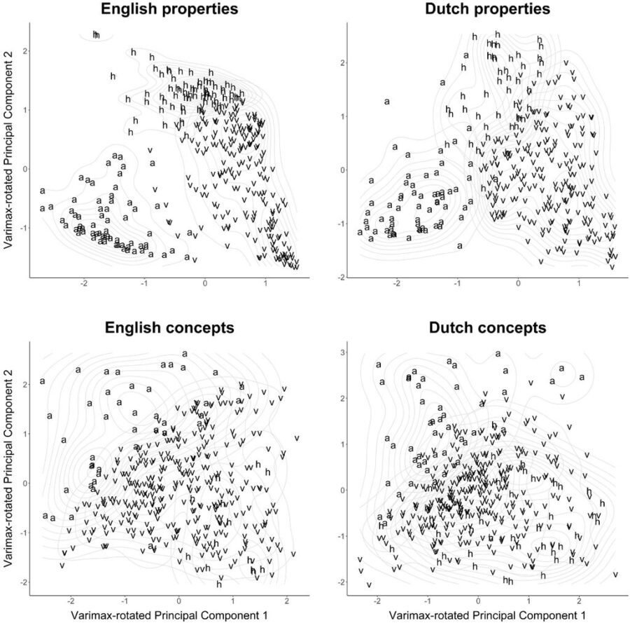
An example of this code is use is available here (with data here).
References
Field, A. P., Miles, J., & Field, Z. (2012). Discovering statistics using R. London: Sage.
For original post, click here.