
This article is in continuation to our previous topic ‘Unsupervised Machine Learning’. Today I’m giving you another powerful tool on this topic named ‘k means Clustering‘. The work in this article is on the continuation of the previous WHO data set featured in ‘Machine Learning: Unsupervised – Hierarchical Clustering and Bootstrapping’. This artifact demonstrates implementing k means clustering and bootstrapping to make sure that the algorithm and clusters formed stand true. The bootstrapping will also evaluate whether we have the right amount of clusters or not and if not what should be the ‘k’ i.e. number of clusters based on ‘Calinski-Harabasz Index’ and ‘Average Silhouette Width (ASW)’. Further, this report relates to how closely identical results are given by k-means with respect to the hierarchical clusters which were formed in the previous post. This is important because, no matter what different algorithms I use for computing clusters, the relation between, the data will remain the same. This indicates clusters should be formed more or less the same (with minimal trade-offs) irrespective of the algorithms used by an individual as data and relationship between the data does not change. Excited?
1. Content Briefing
Following are the contents covered in this article for k-means clustering
- k-means theoretical implementation
- Implementing k-means algorithm in R
- Addressing optimal ‘k’ value using Calinski-Harabasz Index and Average Silhouette Width Index
- Bootstrapping k-means clusters for its validation and confidence
2. The Model
5.1. Data
I have used R language to code for clustering on the World Health Organization (WHO) data, containing 35 countries limited to the region of ‘America’[3]. Following are the data fields:
- $Country: contains names of the countries of region America (datatype: string)
- $Population: contains population count of respective countries (datatype: integer)
- $Under15: count of population under 15 years of age (datatype: number)
- $Over60: count of population over 60 years of age (datatype: number)
- $FertilityRate: fertility rate of the respective countries (datatype: number)
- $LifeExpectancy: Life expectancy of people of respective countries (datatype: integer)
- $CellularSubscribers: Count of people of respective countries possessing cellular subscriptions (datatype: number)
- $LiteracyRate: Rate of Literacy of respective countries (datatype: number)
- $GNI: Gross National Income of respective countries (datatype: number)
5.2. K Means Clustering
K means is another popular clustering algorithm where we try to categorize data based on forming clusters. K means to find it large applications in document classifications, delivery store optimizer, identifying crime localities, customer segmentation, etc. as all the clustering algorithms. So, the question arises how is k-means different? and why do we need it? K means is one of the simplest algorithms to implement when you have the data which is all numeric and the distance metric used in squared Euclidean. It is a high ad hoc algorithm to be used in clustering with only one major disadvantage, any guess?
- Select random number of ‘k’ cluster centers for your data. (this is the disadvantage of k-means clustering that we need to pre-define the number of clusters we need, can lead to unwanted results)
- For the selected centers we now assign all the data points which are nearest to it forming our clusters
- Now, for the clusters formed we compute the centers of the clusters
- Further, we start reassigning the data points as per the new cluster centers we just formed in step 3.
- Steps 3 and 4 are iterative and should be done until no further possibility of trading data points between clusters or you may have reached to maximum number of iterations that might be set.
All of the above steps for building a k means model will be understood clearly with the following figure illustration below:
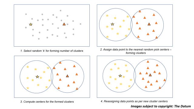
Image illustration for k means clustering
5.4. Practical Implementation
My model for k-means clustering is built on the ‘WHO’ Health data limited to the American region containing 35 countries. This is the same data which was used by me for implementing Hierarchical Clustering. This will also help us understand whether using different algorithms on the same set of data produces the same clusters or different? Thinking logically if the data is the same which means the relationship between the data remains the same, indicating that the weights and distances of the data points in a plane also will be the same. So irrespective of what algorithm we use we should get the same set of clusters. Will we? We’ll figure out very soon. So get ready with your R-Studio and make sure you have the data downloaded from my website. Here is the data download link: https://talktomedata.files.wordpress.com/2019/05/who3.xlsx
5.5. R Algorithm for k-means
5.5.1 Reading and Scaling Data
Moving ahead I have scaled the data, which is a really important aspect to get good clusters and without any flaws. I have scaled data to set mean = 0 and with a standard deviation of 1 for all the data columns except the first one which is ‘Country’. First, I create an object ‘scaling.variables’ for all the columns except the first as I mentioned. Going ahead, I am using scale() function to scale the columns isolated except the first column. The scale function gives two attributes ‘scaled: center’ and ‘scaled: scale’ which are saved into different objects, these objects can be handy if we need to remove the data scaling.
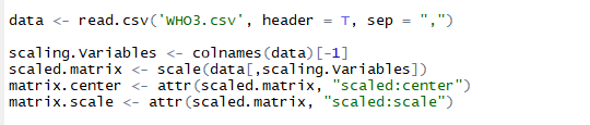
R listing for reading and scaling the data
Printing clusters is crucial and it is not a good idea to print them with all the columns of data as this may be confusing in finding the cluster relations. You have to try combinations of data columns to make sure you are printing the right amount of columns so that you can find a relation between the clusters. To print them I am forming a function named ‘clusters_print’. This will help me print the clusters formed by kmeans() limiting the columns to “Country”, “CellularSubscribers”, “LiteracyRate” and “GNI”. Below is the listing for the clusters_print function.
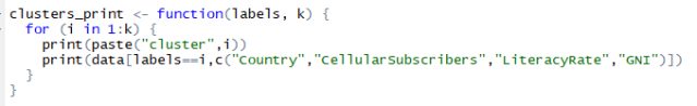
Listing for function to print clusters with limited columns
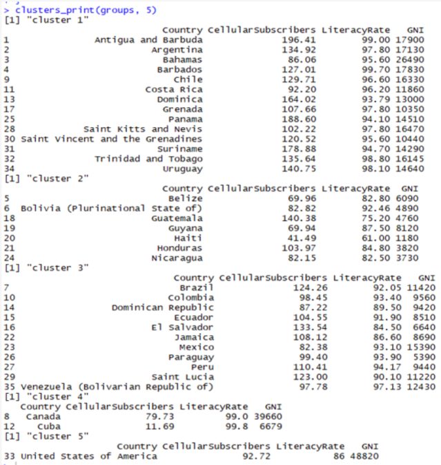
5.5.2 Clustering using kmeans()
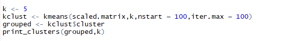
Listing for k-means clusters and printing them
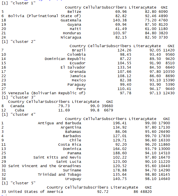
Following can be inferred from the clusters formed above:
- Here, clusters formed are somewhat in relation to the geographic mapping of the countries
- Cluster 1 contains countries with least average GNI all being in 4 figures and literacy rate averaging 80.89
- Cluster 2 is a good mix of countries with 4 and 5 digits GNI along with literacy rate averaging 92.18
- Cluster 3 has countries with highest literacy rate with minimum being 99%
- Cluster 4 too has countries with good literacy rates with minimum being 90% and GNI for all the countries in cluster 4 is in 5 figures
And guess what, these are more or less the same clusters with little trade-offs which were formed in Hierarchical Clusters from my previous blog: Machine Learning: Unsupervised – Hierarchical Clustering and Bootstrapping. Below is the clusters image which was formed in Hierarchical Clustering for comparison purposes.
Clusters formed in Hierarchical clustering (refer Hierarchical clustering blog)
5.5.3. Optimal ‘k’ for Clusters
5.5.3.1. Calinski-Harabasz Index (ch)
The Calinski-Harabasz index of a clustering is the ratio of the between-cluster variance
(which is essentially the variance of all the cluster centroids from the dataset’s grand
centroid) to the total within-cluster variance (basically, the average WSS of the clusters
in the clustering).
5.5.3.2. Average Silhouette Width (asw)
Measures how well an individual data point is clustered and further estimates average distance between clusters. The silhouette plot displays a measure of how close each point in one cluster is to points in the neighboring clusters.
5.5.3.3. Computing ch and asw
kmeansruns() another function in ‘fpc’ package of R can be used to compute Calinski-Harabasz Index (ch) and Average Silhouette Width (asw) automatically. This runs k-means over a range of k and then estimates best k. It further returns the best value of k and output of kmeans for the respective k value. Using kmeansruns() on the scaled data for ‘krange=1:10’ i.e. all values of k from 1 to 10 and criterion = ‘ch’ and ‘asw’ respectively. The kmeansruns() gives the best k value as one of its output that can be extracted as $bestk. Below are the R listing and best value of k obtained.
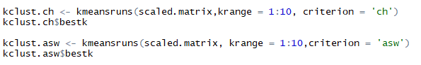
Listing to compute ch and asw using kmeansruns and extracting bestk
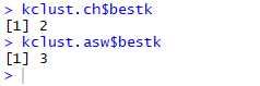
Best k values obtained from ch and asw
The Calinski-Harabasz index gives the best k-value as 2 and Average Silhouette Width gives the best k value as 3. Thus, 2 or 3 is our optimal number of ‘k’ for this data set. Now, you can question me why did I use k = 5? This is simply because in my last blog of Hierarchical Clustering k was 5 so I used the same k here too, to illustrate how close we get the same clusters irrespective of the clustering algorithm that we deploy.
5.5.4. Visual Examination of ‘ch’ and ‘asw’ indexes
As per the listing for computing ‘asw’ and ‘ch’, I have used krange = 1:10. I am now going to compute both the indexes for a range of 1 to 10 against the ‘score’ of individual indexes. The index with the highest score is returned as best ‘k’. I have computed a data-frame that combines criterion values one of the outputs of kmeasnruns() function. Further, I reshape this data frame using the melt() function of R in ‘reshape2’ library. Further using ‘ggplot2’ library I have plotted the data frame. The listing and output are shown below.
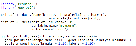
Listing for forming data-frame of combined asw and ch, later plotting them
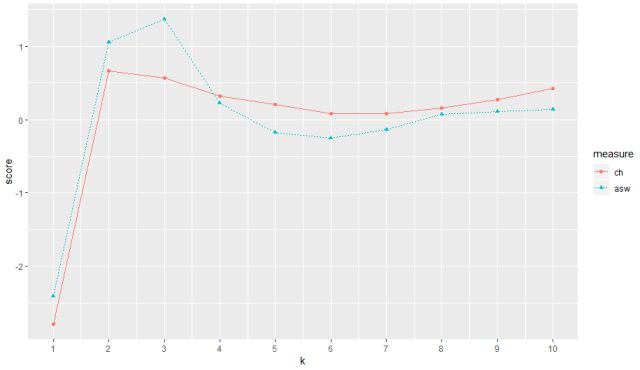
The output for range of indexes from 1-10 of ‘ch’ and ‘asw’
The plot for both ch and asw can be seen in the above figure for a range of k value from 1 to 10. ch (red) peaks at maximum score at 2 thus returning us best k value as 2 and asw peaks best score at index value 3 thus returning us with best k value as 3.
5.5.5 Bootstrapping of k-means
Bootstrapping is the litmus test that our model needs to validate positively so that we can rely on our model and can bet upon its findings and maybe if required test them for unknown data points to predict clusters. Clusterboot() function in ‘fpc’ package does the bootstrapping by re-sampling to evaluate how stable our clusters are. It works on Jaccard co-efficient a similarity measure between sets. Jaccard coefficient values should be greater than 0.5 for all our clusters to make sure our clusters are best formed. For an in-depth explanation and understanding of bootstrapping theory refer to my blog on Hierarchical Clusters.
For the test again I am selecting k = 5 as bestk to evaluate previously formed clusters. Further, using cluster boot on scaled data with arguments as clustermethod = kmeansCBI to indicate kmeans cluster-boot, running it i.e. booting it 100 times and maximum iterations for each booting to be 100. All this to be done for krange of my best k selected i.e. 5 clusters. the seed is set equal to random number 9898 for result reproducibility. We can extract clusters formed by bootstrap in $result$partition of the bootstrap model formed. These clusters are taken in to object ‘groups’ and clusters are printed using the cluster_print function that we formed earlier. Below are the listings and the clusters formed over evaluation of 100 runs and 100 iterations respectively.
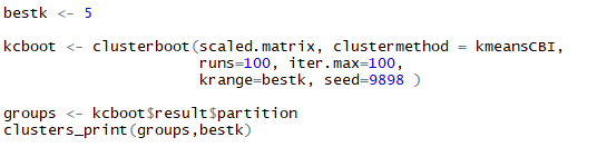
Listing for cluster-boot of k-means and printing them
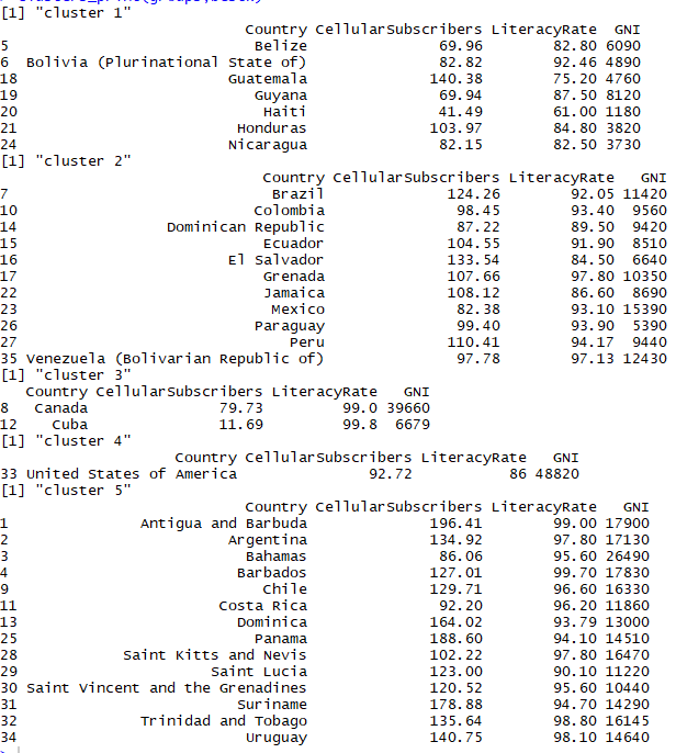
Bootstrap clusters
As we can see above the clusters formed initially in k-means are same as the clusters formed here in bootstraps. This shows that we have fairly stable clusters that can be trusted and deployed in practical use as they pass the test of 100 booting and 100 iterations.
Further, our results obtained in bootstrapping can be rectified by seeing each cluster’s maximum Jaccard Co-efficient which should be greater than 0.5 value indicating stability and number of time on 100 did each cluster dissolved proving its stability. Below is the combined listing and output for Jaccard coefficient and the number of times a cluster dissolved.
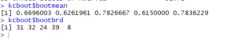
Maximum Jaccard Co-efficient and each cluster dissolution (on 100)
Here, we got all the Jaccard coefficient of all the clusters above 0.6 and a good number for cluster dissolving too in 100 times. These values just give us another layer of confidence on our clusters via bootstrapping.
3. Conclusion
- k-means is one the best and simplest ways to compute unsupervised machine learning with clustering
- Always remember to scale your data preferably with mean 0 and stdv. of 1 for all the numeric data columns for getting clean results
- If required perform ch and asw indexing before computing k-means if you are not sure about what should be your optimal ‘k’ value for k-means clustering
- Always bootstrap your model by trying to produce similar results as original to be confident about your model and findings
7. Clustering Takeaways:
- The goal is simply to draw out similarities by forming a subset of your data.
Good clusters indicate the data points in one cluster are similar and dissimilar to data points in another cluster - Units of data field matter, different units in different respective data fields produce potentially different results, it is always a good idea to have a clear sense of data and data units before clustering
- You will always like the scenario of unit change of output change across categories to represent the same unit change (consistency). Thus, it becomes important that you scale your data as I have scaled with mean set 0 and standard deviation of 1.
- Clustering is always deployed as a data exploration algorithm and can act as a precursor to supervised learning
- Can be considered similar to visualization, with more iterations and interactions you can understand your data better unlike automated machine learning processes like supervised learning
- Many theories to attain best k value for your clusters, the best are indicated here and others too can be explored easily, but it is always wise to choose the best as per the situation
To read the original post, click here
Cheers,
Neeraj