
Users who bought this… Also bought this…‘, I consider this as the statement of this generation. There is not a single shopping application not showcasing this feature to gain more from the buyers. This rule is another by-product of Machine Learning. We humans always look for more similar things which we like for example if a reader starts to like a book of the specific genre say ‘biography’ he/she is leaned towards having more such similar books. And this is what we call ‘associate’. User associates more such books of biography as an interest of reading the genre which he liked and this algorithm is widely used today by shopping sites to recommend users with similar items they liked with what we call as ‘Association Rules’. This not only finds its application to recommend a bundle of things which are bought together or seen together on shopping sites but also this is used to place the bundled items together on the store shelves or maybe to make better navigation to redesign websites.
Understanding Association Rule
As I mentioned it is a by-product of Machine Learning, and is impossible to implement without data. In association, there is a sea of data of user ‘transactions’ and seeing the trend in these transactions that occur more often are then converted into rules. Let’s break it down; ‘Transaction’ can be a single shopping cart, the web pages visited by the user during a web session, in general transactions are actions of our customers and the items/objects which are viewed by the users are referred to as items or item-sets of the transactions. These can also be referred to as cart/baskets/bundles with respect to shopping analogy.
Association Rule Mining is thus based on two set of rules:
- Look for the transactions where there is a bundle or relevance of association of secondary items to the primary items above a certain threshold of frequency
- Convert them into ‘Association Rules’
Let us consider an example of a small database of transactions from a library
| 0. The Hobbit, The Princess Bride |
| 1. The Princess Bride, The Last Unicorn |
| 2. The Hobbit |
| 3. The Never-ending Story |
| 4. The Last Unicorn |
| 5. The Hobbit, The Princess Bride, The Fellowship of the Ring |
| 6. The Hobbit, The Fellowship of the Rings, The Two Towers, The Return of the King |
| 7. The Fellowship of the Ring, The Two Towers, The Return of the King |
| 8. The Hobbit, The Princess Bride, The Last Unicorn |
| 9. The Last Unicorn, The Never-ending Story |
Let us form rules, The Hobbit is in 50% of the transactions in the above listing 5/10. The Princess Bride is 40% of the times 4/10. And both together are bought 30% of the time 3/10. We can say that the support of {The Hobbit, The Princess Bride} is 30%. Out of 5 transactions of The Hobbit 60 % i.e. 3/5 transactions are for The Princess Bride. This 60% is the confidence of the rule we just formed. Thus, we formed a rule that supportThe Hobbit and The Princess bride 30% of the times with confidence being 60%. This states 30% of all the transactions we see are possibly both being bought together. And if The Hobbit is bought, there is 60% chance user might also buy The Princess Bride. Thus, we associate ‘Users who bought The Hobbit, Also bought The Princess Bride’ at the checkout.
The rule is also applicable conversely whenever The Princess Bride was bought 40% of all transactions 4/10. The Hobbit appeared 3 times 3/4 i.e. 75% of the time. Thus, ‘Users who bought The Princess Bride also bought The Hobbit’, for this rule we have support of 30% of all the transactions and confidence of 75%. We can conclude support and confidence form the basis of association rules. To mathematically define support and confidence consider X and Y are our items in Association i.e. ‘Users who bought X also bought Y’ where X is our Primary item and Y is our secondary/associated item. Moving on, we our looking this transaction in a transaction set say, T. With these assumptions we have support S = X + Y / T and confidence C = X / Y. There is always minimal benchmark one should set before forming association rules, I always consider support of minimum of 10% and confidence of minimum of 60%. There is no point of associating with support of 5% with confidence of 20%. It is a waste of rule and time used behind forming such rules, ‘over associations’.
Data for this Algorithm
The data is extracted from the University of Freiburg, from the research they conducted. The data is based on a bookstore database. The data consists of the interests of customers in the books. The information about customer interests in the books is based on their previous purchases and book interests. Purchase is a sign of interest and also the ratings which the users have given also indicates their interest. Thus, for our data transaction is our customers and the item-set is all the books they have expressed interest in, can either be by purchasing or by ratings they left. To implement our rules will be using library package arules and a function in it called apriori, as we cruise further we will better understand the working
Model – Analyzing and Preparing Data
As always the data is available at ‘The Datum’ site and the link is provided in the references section, to download the data for your practice. Refer references at the end of this article. The file is tsv. file which is tab separated values. To read the file, I have used here read.transactions() function of R with some easy to understand arguments listed below. The only thing to note here is read.transactions() reads our file in 2 formats. One where every single row corresponds to a single value and second where each row corresponds to a single transaction, with a possibly unique ID. To read the data in the first format the argument is format=”single” while for the second format argument is format=”basket”. And one more argument to focus upon is to look for and remove the duplicate entries which is done by: rm.duplicates=T. This is done because there is a possibility that user might have bought a book but may have later rated book of a different version which creates a duplicate entry for the same book, thus removing duplicates.
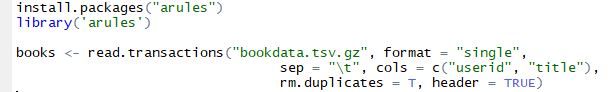
Listing for reading the data and setting up arules library
Further, to understand our data various basic operation are been performed to get the data insights, below is the console view showing the listings used along with respective outputs to get data insights.
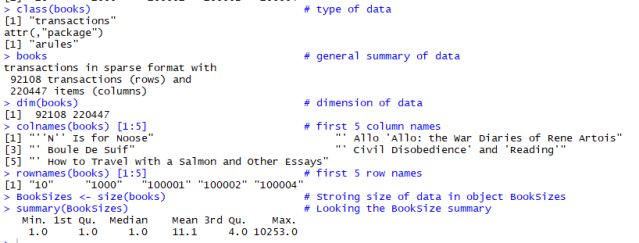
Console view of basic listings for data insights.
text after # are the comments to understand function
The last listing is very interesting, people having interest in mean 11 number of books, but there are some who have shown interest in more 10000 books, let’s spot them! We will now look at the distribution of the BookSizes with an increment of 10% scale and plot it using ggplot function. Below are the listings and output
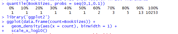
Listing for 10% distribution of data and plotting it
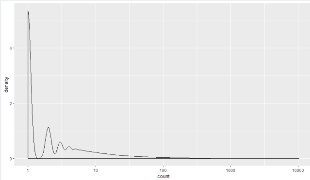
Plot of 10% incremental distribution of data
The above figure indicates the following:
- 90% of customers expressed interest in less than 15 books
- Most of the other groups show interest in close to 100 books
- But still, there are few showing interest in 10000 books or so
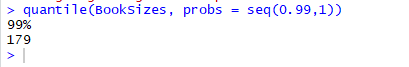
Listing to segregate 99% of interest in number of books
The above shows 99% of customers expressed interest in 179 or fewer number of books
It is now very intuitive to figure out that people showing interests in 1000s of books, which books are they reading? The function in R called itemFrequency() gives us the frequency of each book in transaction data:
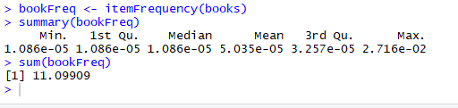
Listing for finding out the frequency of books read w.r.t. transactions
As we can clearly see above the expected frequency should have been summed up to 1, which in our case is not true. We can recover a number of times that each book occurred in the data by normalizing the item frequencies and then multiplying them by the total number of items
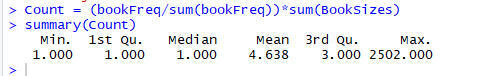
Listing to normalize the frequency of books and summarizing
Now, we will have a look at the ordered books, which will help us know which books were bought more often as we will list the top 10 ordered books. Below is the listing and output.
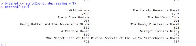
Listing for top 10 most ordered books
As we can see that the most popular book ordered 2502 times is Wild Animus. Now, the point to note, as I mentioned earlier in association support should be minimal of 10% but, there is another rule to follow depending upon the size of your data and also somewhat depending upon your data market (here books). Since we have very large data-set of transactions and also large unique items it is wise to set support of lower values, this is because when we have thousands of unique items (there are a lot of unique books here in the data) the association goes down because the user had thousands of options. Now let’s see what is the % of the order of Wild Animus w.r.t. to the entire data-set.
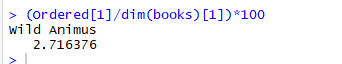
Listing for % order of the highest single book ordered
As we can see above, Wild Animus was bought only almost 3% of the times in entire transactions. Since the highest number of times a single book ordered is close to 3%, the support % is likely to go down in this case.
Here, in the data trend, we noticed more than half of the customers only expressed interest in a single book. This is not our feasible data to associate because for single interests or transaction we cannot actually associate the user likes to other similar books. Thus, we will now refine our data for interests greater than 1 customer.
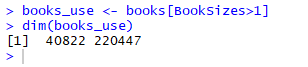
Listing to refine data for customers greater than 1 interests
Model – Applying Association Rules using apriori() function
We are now finally going to apply the association rules, with support and confidence as stated below in the argument of apriori() function listing

Association rule mining using apriori() function
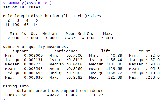
Summary of our rule applied
The summary gives us all the insights into the rules we extracted from the function. There are in all 191 rules that can be associated with our given set of data. Rule length distribution gives us the length of the distinct rules formed. In this case, most rules contain 3 items (100 rules, (with 2 on lhs (X) and one on rhs(Y))). The other aspects, in summary, are the summary of the quality measures of all the rules which are attributed to support, confidence, lift and count. And lastly, some information about how was apriori() applied.
As mentioned earlier, support and confidence are our kind of pillars in forming association rules, but there is more to it, another important aspect called ‘lift’. So what is this? It compares the frequency of an observed pattern with how often you’d expect to see the pattern just by chance. If X then Y lift is equal to
support(Union (X , Y)) / (support(X) * support(Y))
If the lift is near one, it is likely that pattern you are observing is just by chance, the larger the lift, the more likely that the pattern is ‘real’. In our discovered rules 40 is the minimum lift and an average of 105 indicates they are real patterns and not just by chance patterns as they reflect patterns of customer behavior.
Validation of Rules
R gives us some upfront functions from which we can evaluate our rules that we formed using apriori(), the function is known as interestMeasure(). The function helps us measure coverage and fishersExactTest. Coverage supports the left-hand side of the rule i.e. it focuses solely on (X), it gives us an idea about how often the rule will be applied in the dataset. While the latter evaluates whether the observed pattern is real or not. It is the measurement of the probability that you will see the rule by chance, thus we should expect the p-value to be minimal.
Below are the listings and output for coverage and fishersExactTest
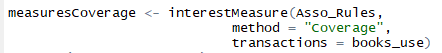
Listing of Measurement for Coverage
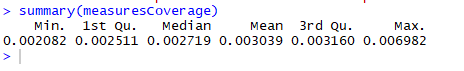
Summary output of Coverage measure
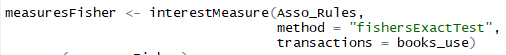
Listing of Measurement for fisherExactTest
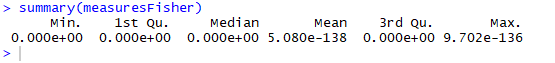
Summary output of fisherExactTest measure
In above, coverage discovered rules from 0.002 to 0.007, which if converted is equivalent range of 100-250 people. And to add to it, all p-values are small so it states that rules reflect actual customer behavior patterns
We can also use R’s inspect() function, it prints the rules. Below is the listing for inspect function using sort, to sort the rules as per our needs
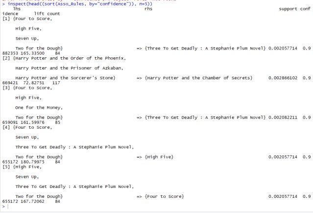
Output for inspect() function, shows lhs and rhs books sorted with confidence
Example: (X) lhs if we pick Four to Score, High Five, Seven Up, and Two for the Dough; customer is likely to pick Three to get Deadly. Support for this rule is 0.002, confidence is 0.988 and Lift measure of 165
One can also restrict which rules to mine, i.e. restrict the X – LHS of the rules to see how many associated rules we have w.r.t. to selected LHS i.e. X. Below is the listing for using apriori() to limit the LHS as ‘The Lovely Bones: A Novel’ with support of 0.001 and confidence of 0.6.
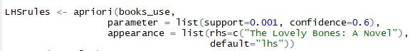
Listing for limiting lhs
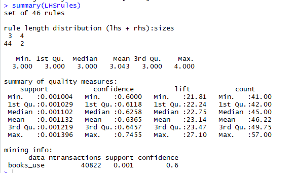
Output of the limited lhs rule
We can see here for the book selected we found: 46 rules
Further, we can again use inspect() and interestMeasures() to evaluate this rule as well
Association Rules Takeaways
- Association rules are based on a single goal to find relations in data or items or attributes that tend to occur together
- If you are not sure that if X then Y is true or occurring just by chance, one should use Lift or Fisher’s Exact test for validation
- When event or data-set is very large, support is tend to be less
- Rules are many, you can sort and choose the one as per the application
To view the original post click here