
This article is inspired by this SIGGRAPH paper by Levin et. al, for which they took this patent , the paper was referred to in the course CS1114 from Cornell. This method is also discussed in the coursera online image processing course by NorthWestern University. Some part of the problem description is taken from the paper itself. Also, one can refer to the implementation provided by the authors in matlab, the following link and the following python implementation in github.
The Problem
Colorization is a computer-assisted process of adding color to a monochrome image or movie. In the paper the authors presented an optimization-based colorization method that is based on a simple premise: neighboring pixels in space-time that have similar intensities should have similar colors.
This premise is formulated using a quadratic cost function and as an optimization problem. In this approach an artist only needs to annotate the image with a few color scribbles, and the indicated colors are automatically propagated in both space and time to produce a fully colorized image or sequence.
In this article the optimization problem formulation and the way to solve it to obtain the automatically colored image will be described for the images only.
The Algorithm
YUV/YIQ color space is chosen to work in, this is commonly used in video, where Y is the monochromatic luminance channel, which we will refer to simply as intensity, while Uand V are the chrominance channels, encoding the color.
The algorithm is given as input an intensity volume Y(x,y,t) and outputs two color volumes U(x,y,t) and V(x,y,t). To simplify notation the boldface letters are used (e.g. r,s) to denote ") triplets. Thus, Y(r) is the intensity of a particular pixel.
triplets. Thus, Y(r) is the intensity of a particular pixel.
Now, One needs to impose the constraint that two neighboring pixels r,s should have similar colors if their intensities are similar. Thus, the problem is formulated as the following optimization problem that aims to minimize the difference between the colorU(r) at pixel r and the weighted average of the colors at neighboring pixels, where w(r,s)is a weighting function that sums to one, large when Y(r) is similar to Y(s), and small whenthe two intensities are different.

When the intensity is constant the color should be constant, and when the intensity is an edge the color should also be an edge. Since the cost functions are quadratic and
the constraints are linear, this optimization problem yields a large, sparse system of linear equations, which may be solved using a number of standard methods.
As discussed in the paper, this algorithm is closely related to algorithms proposed for other tasks in image processing. In image segmentation algorithms based on normalized cuts [Shi and Malik 1997], one attempts to find the second smallest eigenvector of the matrix D − W where W is a npixels×npixels matrix whose elements are the pairwise affinities between pixels (i.e., the r,s entry of the matrix is w(r,s)) and D is a diagonal matrix whose diagonal elements are the sum of the affinities (in this case it is always 1). The second smallest eigenvector of any symmetric matrix A is a unit norm vector x that minimizes  and is orthogonal to the first eigenvector. By direct inspection, the quadratic form minimized by normalized cuts is exactly the cost function J, that is
 x =J(x)") . Thus, this algorithm minimizes the same cost function but under different constraints. In image denoising algorithms based on anisotropic diffusion[Perona and Malik 1989; Tang et al. 2001] one often minimizes a function
. Thus, this algorithm minimizes the same cost function but under different constraints. In image denoising algorithms based on anisotropic diffusion[Perona and Malik 1989; Tang et al. 2001] one often minimizes a function
similar to equation 1, but the function is applied to the image intensity as well.
The following figures show an original gray-scale image and the marked image with color-scribbles that are going to be used to compute the output colored image.
Original Gray-scale Image Input

Gray-scale image Input Marked with Color-Scribbles

Implementation of the Algorithm
Here are the the steps for the algorithm:
- Convert both the original gray-scale image and the marked image (marked with color scribbles for a few pixels by the artist) to from RGB to YUV / YIQ color space.
- Compute the difference image from the marked and the gray-scale image. The pixels that differ are going to be pinned and they will appear in the output, they are directly going to be used as stand-alone constraints in the minimization problem.
- We need to compute the weight matrix W that depends on the similarities in the neighbor intensities for a pixel from the original gray-scale image.
- The optimization problem finally boils down to solving the system of linear equations of the form
 that has a closed form least-square solution
. Same thing is to be repeated for the V channel too. - However the W matrix is going to be very huge and sparse, hence sparse-matrix based implementations must be used to obtain an efficient solution. However, in this python implementation in github, the scipy sparse lil_matrixwas used when constructing the sparse matrices, which is quite slow, we can construct more efficient scipy csc matrix rightaway, by using a dictionary to store the weights initially. It is much faster. The python code in the next figure shows my implementation for computing the weight matrix W.
- Once W is computed it’s just a matter of obtaining the least-square solution, by computing the pseudo-inverse, which can be more efficiently computed with LU factorization and a sparse LU solver, as in this python implementation in github.
- Once the solution of the optimization problem is obtained in YUV / YIQ space, it needs to be converted back to RGB. The following formula is used for conversion.
 that has a closed form least-square solution
}^{-1}W^{T}b") . Same thing is to be repeated for the V channel too.
. Same thing is to be repeated for the V channel too.
|
1
2
3
4
5
6
7
8
9
10
11
12
13
14
15
16
17
18
19
20
21
22
23
24
25
26
27
28
29
|
import scipy.sparse as spfrom collections import defaultdictdef compute_W(Y, colored): (w, h) = Y.shape W = defaultdict() for i in range(w): for j in range(h): if not (i, j) in colored: # pixel i,j in color scribble (N, sigma) = get_nbrs(Y, i, j, w, h) #r = (i, j) Z = 0. id1 = ij2id(i,j,w,h) # linearized id for (i1, j1) in N: #s = (i1, j1) id2 = ij2id(i1,j1,w,h) W[id1,id2] = np.exp(-(Y[i,j]-Y[i1,j1])**2/(sigma**2)) if sigma > 0 else 0. Z += W[id1,id2] if Z > 0: for (i1, j1) in N: #s = (i1, j1) id2 = ij2id(i1,j1,w,h) W[id1,id2] /= -Z for i in range(w): for j in range(h): id = ij2id(i,j,w,h) W[id,id] = 1. rows, cols = zip(*(W.keys())) #keys data = W.values() #[W[k] for k in keys] return sp.csc_matrix((data, (rows, cols)), shape=(w*h, w*h)) #W |
Results
The following images and animations show the results obtained with the optimization algorithm. Most of the following images are taken from the paper itself.
Original Gray-scale Image Input Gray-scale image Input Marked
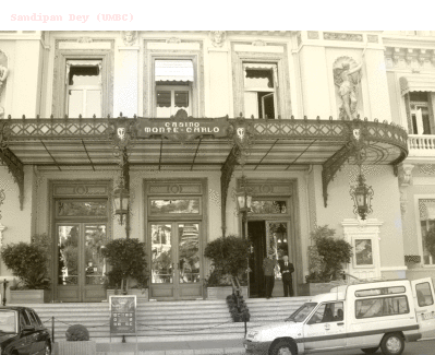
Color image Output

The next animations show how the incremental scribbling results in better and better color images.
Original Gray-scale Image Input

As can be seen from the following animation, the different parts of the building get colored as more and more color-hints are scribbled / annotated.
Gray-scale image Input Marked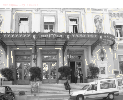
Color image Output
Original Gray-scale Image Input

Gray-scale image Input Marked
Color image Output
Original Gray-scale Image Input (me)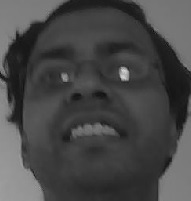
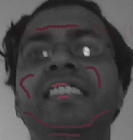
Gray-scale image Input Marked incrementally
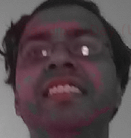
Color image Output
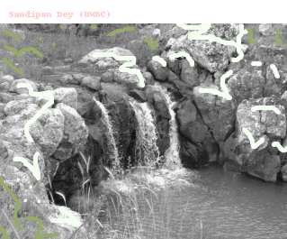
Original Gray-scale Image Input

Gray-scale image Input Marked

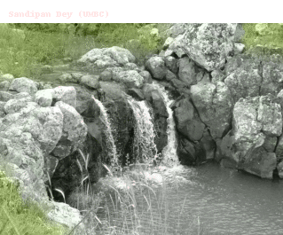
Color image Output

Original Gray-scale Image Input

Gray-scale image Input Marked
 https://sandipanweb.files.wordpress.com/2018/01/madurga_gray_marked… 150w” sizes=”(max-width: 413px) 100vw, 413px” />
Color image Output
