
In this continuation of “Hybrid content-based and collaborative filtering recommendations wi…” I will describe the application of the {ordinal} clm() function to test a new, hybrid content-based, collaborative filtering approach to recommender engines by fitting a class of ordinal logistic (aka ordered logit) models to ratings data from the MovieLens 100K dataset. All R code used in this project can be obtained from the respective GitHub repository; the chunks of code present in the body of the post illustrate the essential steps only. The MovieLens 100K dataset can be obtained from the GroupLens research laboratory of the Department of Computer Science and Engineering at the University of Minnesota. This second part of the study relies on the R code in OrdinalRecommenders_3.R and presents the model training, cross-validation, and the analyses. But before we proceed to approach the recommendation problem from a viewpoint of discrete choice modeling, let me briefly remind you of the results of the feature engineering phase and explain what happens in OrdinalRecommenders_2.R which prepares the data frames that are passed to clm().
Enter explanatory variables
In the feature engineering phase (OrdinalRecommender_1.R) we have produced four – two user-user and two item-item – matrices. Of these four matrices, two are proximity matrices with Jaccard distances derived from binarized content-based features: for users, we have used the binary-featured vectors that describe each user by what movies he or she has or has not rated, while for items we have derived the proximity matrix from the binarized information on movie genre and the decade of the production. In addition, we have two Pearson correlation matrices derived from the ratings matrix directly, one describing the user-user similarity and the other the similarity between the items. The later two matrices present the memory-based component of the model, while the former carry content-based information. In OrdinalRecommenders_2.R, these four matrices are:
- usersDistance – user-user Jaccard distances,
- UserUserSim, – user-user Pearson correlations,
- itemsDistance – item-item Jaccard distances, and
- ItemItemSim – item-item Pearson correlations.
The OrdinalRecommenders_2.R essentially performs only the following operations over these matrices: for each user-item ratings present in ratingsData (the full ratings matrix),
- from the user-user proximity/similarity matrix, select 100 most users who have rated the item under consideration and who are closest to the user under consideration;
- place them in increasing order of distance/decreasing order of similarity from the current user;
- copy their respective ratings of the item under consideration.
For the item-item matrices, the procedure is similar:
- from the item-item proximity/similarity matrix, select 100 items that the user under consideration has rated and that are closest to the item under consideration;
- place them in increasing order of distance/decreasing order of similarity from the current item;
- copy the respective ratings of the item under consideration.
Note that this procedure of selecting the nearest neighbours’ ratings produces missing data almost by necessity: a particular user doesn’t have to have 100 ratings of the items similar to the item under consideration, and for a particular user and item we don’t necessarily find 100 similar users’ ratings of the same item. This would reflect in a decrease of the sample size as one builds progressively more and more feature-encompassing ordered logit models. In order to avoid this problem, I have first reduced the sample size so to keep only complete observations for the most feature-encompassing model that I have planned to test: the one relying on 30 nearest neighbors from all four matrices (e.g., encompassing 4 * 30 = 120 regressors, add four intercepts needed for the ordered logit over a 5-point rating scale); 87,237 observations from the dataset were kept.
For the sake of completeness, I have also copied the respective distance and similarity measures from the matrices; while the first 100 columns of the output matrices present ratings only, the following 100 columns are the respective distance/similarity measures. The later will not be used in the remainder of the study. The resulting four matrices are:
- proxUsersRatingsFrame – for each user-item combination in the data set, these are the ratings of the item under consideration from the 100 closest neighbours in the user-user content-based proximity matrix;
- simUsersRatingsFrame, – for each user-item combination in the data set, these are the ratings of the item under consideration from the 100 closest neighbours in the user-user memory-based similarity matrix;
- proxItemsRatingsFrame – for each user-item combination in the data set, these are the ratings from the user under consideration of the 100 closest neighbours in the item-item content-based proximity matrix; and
- simItemsRatingsFrame – for each user-item combination in the data set, these are the ratings from the user under consideration of the 100 closest neighbours in the item-item memory-based similarity matrix.
Of course it can be done faster than for-looping over 100,000 ratings. Next, the strategy. The strategy here is to progressively select a larger number of numSims – the number of nearest neighboours taken from proxUsersRatingsFrame, simUsersRatingsFrame, proxItemsRatingsFrame, and simItemsRatingsFrame – and pull them together with the ratings from the ratingsData. For example, if numSims == 5, we obtain a predictive model Rating ~ 4 matrices * 5 regressors which is 20 regressors in total, if numSims == 10, we obtain a predictive model Rating ~ 4 matrices * 10 regressors which is 40 regressors in total, etc.
Enter Ordered Logit Model
The idea to think of the recommendation problem as discrete choice is certainly not new; look at the very introductory lines of [1] where the Netflix competition problem was used to motivate the introduction of ordered regressions in discrete choice. We assume that each user has an unobservable, continuous utility function that maps onto his or her item preferences, and of which we learn only by observing the discrete information that is captured by his or her ratings on a 5-point scale. We also assume that the mapping of the underlying utility on the categories of the rating scale is controlled by threshold parameters, of which we fix the first to have a value of zero, and estimate the thresholds for 1→2, 2→3, 3→4, and 4→5 scale adjustments; these play a role of category-specific intercepts, and are usually considered as nuisance parameters in ordered logistic regression. In terms of the unobserved user’s utility for items, these threshold parameters “disect” the hypothesized continuous utility scale into fragments that map onto the discrete rating responses (see Chapter 3, Chapter 4.8 in [1]). Additionally, we estimate a vector of regression coefficients, β, one for each explanatory variable in the model: in our case, the respective ratings from the numSims closest neighbours from the similarity and proximity matrices as described in the previous section. In the ordered logit setting – and with the useful convention of writing minus in front of the xiTβ term used in {ordinal} (see [2]) – we have:
![]()
and given that
![]()
the logit is cumulative; θj stands for the j-th response category-specific threshold, while i is the index of each observation in the dataset. Vectors x and β play the usual role. The interpretation of the regression coefficients in β becomes clear after realizing that the cumulative odds ratios take the form of:
![]()
and is independent of the response category j, so that for a unit change in x the cumulative odds ratio of the change in probability P(Yi ≥ j) increases by a multiplicative factor of exp(β). Back to the recommendation problem: by progressively adding more nearest neighbours’’ ratings from the user-user and item-item proximity and similarity matrices, and tracking the behavior of regression coefficients in predictions from the respective ordered logit models, one can figure out the relative importance of the memory-based information (from the similarity matrices) and the content-based information (from proximity matrices).
I have varied the numSims (the number of nearest neighbours used) as seq(5, 30, by = 5) to develop six ordinal models with 20, 40, 60, 80, 100, and 120 regressors respectively, and performed a 10-fold cross-validation over 87,237 user-item ratings from MovieLens 100K (OrdinalRecommenders_3.R):
### --- 10-fold cross-validation for each:
### --- numSims <- seq(5, 30, by = 5)
 numSims <- seq(5, 30, by = 5)
 meanRMSE <- numeric(length(numSims))
 totalN <- dim(ratingsData)[1]
 n <- numeric()
 ct <- 0
 ## -- Prepare modelFrame:
 # - select variables so to match the size needed for the most encompassing clm() model:
 f1 <- select(proxUsersRatingsFrame,
              starts_with('proxUsersRatings_')[1:numSims[length(numSims)]])
 f2 <- select(simUsersRatingsFrame,
              starts_with('simUsersRatings_')[1:numSims[length(numSims)]])
 f3 <- select(proxItemsRatingsFrame,
              starts_with('proxItemsRatings_')[1:numSims[length(numSims)]])
 f4 <- select(simItemsRatingsFrame,
              starts_with('simItemsRatings_')[1:numSims[length(numSims)]])
 # - modelFrame:
 mFrame <- cbind(f1, f2, f3, f4, ratingsData$Rating)
 colnames(mFrame)[dim(mFrame)[2]] <- 'Rating'
 # - Keep complete observations only;
 # - to match the size needed for the most encompassing clm() model:
 mFrame <- mFrame[complete.cases(mFrame), ]
 # - store sample size:
 n <- dim(mFrame)[1]
 # - Rating as ordered factor for clm():
 mFrame$Rating <- factor(mFrame$Rating, ordered = T)
 # - clean up a bit:
 rm('f1', 'f2', 'f3', 'f4'); gc()
 ## -- 10-fold cross-validation
 set.seed(10071974)
 # - folds:
 foldSize <- round(length(mFrame$Rating)/10)
 foldRem <- length(mFrame$Rating) - 10*foldSize
 foldSizes <- rep(foldSize, 9)
 foldSizes[10] <- foldSize + foldRem
 foldInx <- numeric()
 for (i in 1:length(foldSizes)) {
   foldInx <- append(foldInx, rep(i,foldSizes[i]))
 }
 foldInx <- sample(foldInx)
 # CV loop:
 for (k in numSims) {

   ## -- loop counter
   ct <- ct + 1

   ## -- report
   print(paste0("Ordinal Logistic Regression w. ",
                k, " nearest neighbours running:"))

   ### --- select k neighbours:
   modelFrame <- mFrame[, c(1:k, 31:(30+k), 61:(60+k), 91:(90+k))]
   modelFrame$Rating <- mFrame$Rating

   # - model for the whole data set (no CV):
   mFitAll <- clm(Rating ~ .,
                  data = modelFrame)
   saveRDS(mFitAll, paste0("OrdinalModel_NoCV_", k, "Feats.Rds"))

   RMSE <- numeric(10)
   for (i in 1:10) {
     # - train and test data sets
     trainFrame <- modelFrame[which(foldInx != i), ]
     testFrame <- modelFrame[which(foldInx == i), ]
     # - model
     mFit <- clm(Rating ~ .,
                 data = trainFrame)

     # - predict test set:
     predictions <- predict(mFit, newdata = testFrame,
                            type = "class")$fit

     # - RMSE:
     dataPoints <- length(testFrame$Rating)
     RMSE[i] <-
       sum((as.numeric(predictions)-as.numeric(testFrame$Rating))^2)/dataPoints
     print(paste0(i, "-th fold, RMSE:", RMSE[i]))
   }

   ## -- store mean RMSE over 10 folds:
   meanRMSE[ct] <- mean(RMSE)
   print(meanRMSE[ct])

   ## -- clean up:
   rm('testFrame', 'trainFrame', 'modelFrame'); gc()
 }
The outer loop varies k in numSims, the number of nearest neighbours selected, then prepares the dataset, picks ten folds for cross-validation, and fits the ordered logit to the whole dataset before the cross-validation; the inner loop performs a 10-fold cross-validation and stores the RMSE from each test fold; the average RMSE from ten folds for each k in numSims is recorded. This procedure is later modified to test models that work with proximity or similarity matrices exclusively.
Results
The following figure presents the average RMSE from 10-fold CV after selecting 5, 10, 15, 20, 25, and 30 nearest neighbours from the user-user and item-item proximity and similarity matrices. Once again, the similarity matrices represent the memory-based information, while the proximity matrices carry the content-based information. The four different sources of features are termed “feature categories” in the graph.
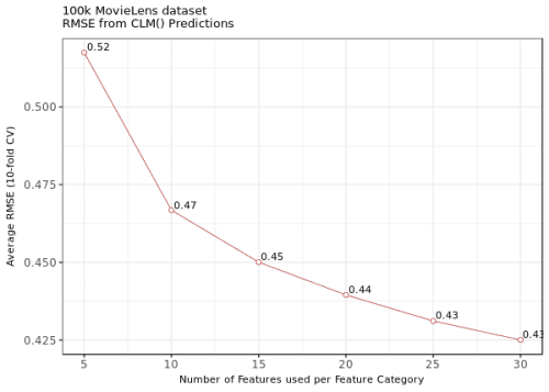
Figure 1. The average RMSE from the 10-fold cross-validations from clm() with 5, 10, 15, 20, 25, and 30 nearest neighbours.
The model with 20 features only and exactly 24 parameters (4 intercepts were estimated plus the coefficients for 5 ratings from four matrices) achieves an average RMSE of around .52. For comparison, in a recent 10-fold cross-validation over MovieLens 100K with {recomme… the CF algorithms achieved an RMSE of .991 with 100 nearest neighbours in user-based CF, and an RMSE of .940 with 100 nearest neighbours in item-based CF: our approach almost double downs the error with a fivefold reduction in the number of features used. With 120 features (30 nearest neighbours from all four matrices) and 124 parameters, the models achieves a RMSE of approximately .43. With these results, the new approach surpasses many recommender engines that were tested on MovieLens 100K in the previous years; for example, compare the results presented here – taking into consideration the fact that the model with 20 features only achieves an RMSE of .517 on the whole dataset (ie. without cross-validation) – with the results from the application of several different approaches presented by the Recommender Systems project of the Carleton College, Northfield, MN.
What about the relative importance of memory and content-based information in the prediction of user ratings? The following figure presents the median values and range of exp(β) for progressively more complex ordinal models that were tested here:
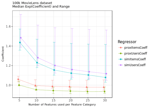
Figure 2. The median exp(β) from the clm() ordered logit models estimated without cross-validation and encompassing 5, 10, 15, 20, 25, and 30 nearest neighbours from the memory-based and content-based matrices.
As it is readily observed, the memory-based features (simItemsCoeff for item-item similarity neighbours, and simUsersCoeff for user-user similarity neighbours in the graph legend) weigh more heavily in the ratings prediction than the content-based features (proxItemsCoeff for the item-item proximity neighbours, and proxUsersCoeff for the user-user proximity neighbours). I have performed another round of the experiment by fitting ordinal models with the information from the memory-based, similarity matrices only; Figure 3 presents the average RMSE obtained from 10-fold CVs of these models:
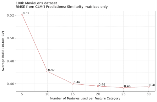
Figure 3. The average RMSE from the 10-fold cross-validations from clm() with 5, 10, 15, 20, 25, and 30 nearest neighbours for models with memory-based information only.
The results seem to indicate almost no change in the RMSEs across the models (but note how the model starts overfitting when more than 25 features per matrix are used). Could it be that the content-based information – encoded by the proximity matrices – is not a necessary ingredient in my predictive model at all? No. But we will certainly not use RMSE to support this conclusion:
modelFiles <- list.files()
modelRes <- matrix(rep(0,6*7), nrow = 6, ncol = 7)
 numSims <- seq(5, 30, by = 5)
 ct = 0
 for (k in numSims) {
   ct = ct + 1
   fileNameSimProx <- modelFiles[which(grepl(paste0("CV_",k,"F"), modelFiles, fixed = T))]
   modelSimProx <- readRDS(fileNameSimProx)
   fileNameSim <- modelFiles[which(grepl(paste0("Sim_",k,"F"), modelFiles, fixed = T))]
   modelSim <- readRDS(fileNameSim)
   testRes <- anova(modelSimProx, modelSim)
   modelRes[ct, ] <- c(testRes$no.par, testRes$AIC, testRes$LR.stat[2],
                       testRes$df[2], testRes$`Pr(>Chisq)`[2])
 }
 modelRes <- as.data.frame(modelRes)
 colnames(modelRes) <- c('Parameters_Model1', 'Parameters_Model2',
                         'AIC_Model1', 'AIC_Model2',
                         'LRTest','DF','Pr_TypeIErr')
 write.csv(modelRes, 'ModelSelection.csv')
The results of the likelihood ratio tests, together with the values of the Akaike Information Criterion (AIC) for all models are provided in Table 1; a comparison between the AIC values are provided in Figure 4. I have compared the models that encompass both the top neighbours from the memory and the content-based matrices, on one, with the models encompassing only information from the memory-based matrices, on the other hand. As you can see, the AIC is consistently lower for the models that incorporate both the content and the memory-based information (with the significant LRTs testifying that the contribution of content-based information cannot be rejected).
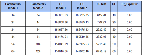
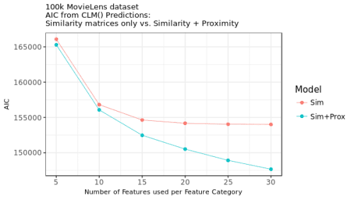
Figure 4. Model selection: AIC for ordered logit models with 5, 10, 15, 20, 25, and 30 nearest neighbours: memory-based information only (Sim) vs. memory-based and content-based models (Sim+Prox).
Summary
Some say that comparing model-based recommendation systems with the CF approaches is not fair in the first place. True. However, achieving a reduction in error of almost 50% by using 80% less features is telling. I think the result has two important stories to tell, in fact. The first one is that the comparison is really not fair :-). The second story is, however, much more important. It is not about the application of the relevant model; since the development of discrete choice models in economics, many behavioral scientist who see a Likert type response scale probably tends to think of some appropriate ordinal model for the problem at hand. It is about the formulation of the problem: as ever in science, the crucial question turns out to be the one on the choice of the most relevant description of the problem; in cognitive and data science, the question of what representation enables for its solution by as simple as possible means of mathematical modeling.
References
[1] Greene, W. & Hensher, D. (2010). Modeling Ordered Choices. Cambridge University Press, 2010.
[2] Christensen, R. H. B. (June 28, 2015). Analysis of ordinal data with cumulative link models – estimation with the R-package ordinal. Accessed on March 03, 2017, from the The Comprehensive R Archive Network. URL: https://cran.r-project.org/web/packages/ordinal/vignettes/clm_intro…
:%20Recommendation%20as%20discrete%20choice)