How to get CAPM in the stock market & equity beta

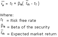
The general idea behind CAPM is that investors need to be compensated in two ways: time value of money and risk. The time value of money is represented by the risk-free (rf) rate in the formula and compensates the investors for placing money in any investment over a period of time. The other half of the formula represents risk and calculates the amount of compensation the investor needs for taking on additional risk. This is calculated by taking a risk measure (beta) that compares the returns of the asset to the market over a period of time and to the market premium (Rm-Rf).

(1) Data Gathering: We are going to gather the market data from the API.
(2) Data Manipulation: We choose only Top 20 firms in terms of market cap.
(3) Data Visulaization: Draw the risk-return graph
(4) Data Interpretation: See this graph is consistent with CAPM theory.

Codes

#NASDAQ, NYSE
market <- “NYSE”
#Technology, Finance, Energy, Consumer Services, Transportation, Capital Goods, Health Care, Basic Industries
sector <- “Technology”

getcapm <- function(stock) {
    #Getting data from server
 
    data <- get.hist.quote(stock, #Tick mark
                           start=”2016-03-01″, #Start date YYYY-MM-DD
                           end=”2016-03-31″ #End date YYYY-MM-DD
    )
 
    #We only take into account “Closing price”, the price when the market closes
    yesterdayprice <- data$Close
    #This is a unique feature of R better than Excel
    #I need to calculate everyday return
    #The stock return is defined as (today price – yesterday price)/today price
    todayprice <- lag(yesterdayprice)
    #ret <- log(lag(price)) – log(price)
    rets <- (todayprice – yesterdayprice)/todayprice
    #Annualized and percentage
    vol <- sd(rets) * sqrt(length(todayprice))
 
    #Getting Geometric Mean.
    #You might be tempted to use just mean(). Don’t do that in stock market.
    geometric_mean_return_prep <- rets + 1
    geometric_mean_return_prep <-  data.frame(Date=time(geometric_mean_return_prep), geometric_mean_return_prep, check.names=FALSE, row.names=NULL)
    geometric_mean_return = 1
 
    for(i in 1:length(geometric_mean_return_prep)) {
        geometric_mean_return = geometric_mean_return * geometric_mean_return_prep[i,2]
    }
    geometric_mean_return <- geometric_mean_return^(1/length(geometric_mean_return_prep))
 
    geometric_mean_return <- geometric_mean_return -1
 
    information <- c(geometric_mean_return, vol) #It’s a trick to return multiple values in one return.
    return(information)
}

convert_marketcap <- function(str) {
    str <- gsub(“\\$”, “”, str) #Get rid of “$” first
    #The reason why I use \\ is that $ has a special meaning in regular expression
    #Regular expression is not the topic. #I’ll deal with later
    multiplier <- str_sub(str,-1,-1) #Million? Billion?
    pure_number <- as.numeric(gsub(“(B|M)”, “”, str)) #Get rid of M or B. Turn it into number
    if(multiplier == “B”) {
        #Billion
        adjustment <- 1000000000
    } else if(multiplier == “M”) {
        #Million
        adjustment <- 1000000
    } else {
        #Don’t adjust it.
        adjustment <- 1
    }
    return (pure_number * adjustment)
}

original <- stockSymbols()

#Getting NASDAQ
listings <- original[original$Exchange==market,]
#As these data include “NA,” we need to clean them up for further data manipulation.
#If you don’t clean up NA, you would encounter error while manipulating
listings <- listings[!is.na(listings$MarketCap),]
listings <- listings[!is.na(listings$Sector),]
#I want to focus on the specific sector
listings <- listings[listings$Sector==sector,]

#Market cap is string right now. We need to convert this to number
listings$MarketCap <- sapply(listings$MarketCap, convert_marketcap)

#Sort the list descending order of market capital
listings <- arrange(listings, desc(listings$MarketCap))

capm <- data.frame(ticker=””, volatility=1:20, geometric_return=1:20)
capm$ticker <- listings$Symbol[1:20]

for(i in 1:20) {
    information_on_stock <- getcapm(capm$ticker[i])
    capm$geometric_return[i] <- information_on_stock[1]
    capm$volatility[i] <- information_on_stock[2]
}

main_name <- paste(market, ” / “)
main_name <- paste(main_name, sector)
main_name <- paste(main_name, ” in Mar 2015″)

capm_regression<-lm(capm$geometric_return ~ capm$volatility)

plot(x=capm$volatility,y=capm$geometric_return,pch=19, main = main_name, xlab=”Stock Volatility”, ylab=”Stock Return”)
#I want to know which stock is outlier.
textxy(capm$volatility, capm$geometric_return, capm$ticker)
abline(capm_regression, col=”red”) # regression line (y~x)

print(summary(capm_regression))

Outcome Interpretation

So, thus remaining things are two – Alpha and Beta.