
In this article, an implementation of an efficient graph-based image segmentation technique will be described, this algorithm was proposed by Felzenszwalb et. al. from MIT. The slides on this paper can be found from Stanford Vision Lab.. The algorithm is closely related to Kruskal’s algorithm for constructing a minimum spanning tree of a graph, as stated by the author and hence can be
implemented to run in O(m log m) time, where m is the number of edges in the graph.
Problem Definition and the basic idea (from the paper)
- Let G = (V, E) be an undirected graph with vertices vi ∈ V, the set of elements to be segmented, and edges (vi, vj ) ∈ E corresponding to pairs of neighboring vertices. Each edge (vi, vj ) ∈ E has a corresponding weight w((vi, vj)), which is a non-negative measure of the dissimilarity between neighboring elements vi and vj.
-
In the case of image segmentation, the elements in V are pixels and the weight of an edge is some measure of the dissimilarity between the two pixels connected by that edge (e.g., the difference in intensity, color, motion, location or some other local attribute).
-
Particularly for the implementation described here, an edge weight functionbased on the absolute intensity difference (in the yiq space) between the pixels connected by an edge, w((vi, vj )) = |I(pi) − I(pj )|.
-
In the graph-based approach, a segmentation S is a partition of V into components
such that each component (or region) C ∈ S corresponds to a connected component
in a graph G0 = (V, E0), where E0 ⊆ E. -
In other words, any segmentation is induced by a subset of the edges in E. There are different ways to measure the quality of a segmentation but in general we want the elements in a component to be similar, and elements in different components to be dissimilar.
-
This means that edges between two vertices in the same component should have relatively low weights, and edges between vertices in different components should have higher weights.
-
The next figure shows the steps in the algorithm. The algorithm is very similar to Kruskal’s algorithm for computing the MST for an undirected graph.

-
The threshold function τ controls the degree to which the difference between two
components must be greater than their internal differences in order for there to be
evidence of a boundary between them. -
For small components, Int(C) is not a good estimate of the local characteristics of the data. In the extreme case, when |C| = 1, Int(C) = 0. Therefore, a threshold function based on the size of the component, τ (C) = k/|C| is needed to be used, where |C| denotes the size of C, and k is some constant parameter.
-
That is, for small components we require stronger evidence for a boundary. In practice k sets a scale of observation, in that a larger k causes a preference for larger components.
-
In general, a Gaussian filter is used to smooth the image slightly before computing the edge weights, in order to compensate for digitization artifacts. We always use a Gaussian with σ = 0.8, which does not produce any visible change to the image but helps remove artifacts.
-
The following python code shows how to create the graph.
|
1
2
3
4
5
6
7
8
9
10
11
12
13
14
15
16
17
18
19
20
21
22
23
24
25
26
27
28
29
30
|
import numpy as npfrom scipy import signalimport matplotlib.image as mpimgdef gaussian_kernel(k, s = 0.5): # generate a (2k+1)x(2k+1) gaussian kernel with mean=0 and sigma = s probs = [exp(-z*z/(2*s*s))/sqrt(2*pi*s*s) for z in range(-k,k+1)]return np.outer(probs, probs)def create_graph(imfile, k=1., sigma=0.8, sz=1): # create the pixel graph with edge weights as dissimilarities rgb = mpimg.imread(imfile)[:,:,:3] gauss_kernel = gaussian_kernel(sz, sigma) for i in range(3): rgb[:,:,i] = signal.convolve2d(rgb[:,:,i], gauss_kernel, boundary='symm', mode='same') yuv = rgb2yiq(rgb) (w, h) = yuv.shape[:2] edges = {} for i in range(yuv.shape[0]): for j in range(yuv.shape[1]): #compute edge weight for nbd pixel nodes for the node i,j for i1 in range(i-1, i+2): for j1 in range(j-1, j+2): if i1 == i and j1 == j: continue if i1 >= 0 and i1 = 0 and j1 < h: wt = np.abs(yuv[i,j,0]-yuv[i1,j1,0]) n1, n2 = ij2id(i,j,w,h), ij2id(i1,j1,w,h) edges[n1, n2] = edges[n2, n1] = wt return edges |
Some Results
- The images are taken from the paper itself or from the internet. The following figures and animations show the result of segmentation as a result of iterative merging of the components (by choosing least weight edges), depending on the internal difference of the components.
- Although in the paper the author described the best value of the parameter k to be around 300, but since in this implementation the pixel RGB values are normalized (to have values in between 0 – 1) and then converted to YIQ values and the YIQ intensities are used for computing the weights (which are typically very small), the value of k that works best in this scenario is 0.001-0.01.
- As we can see from the below results, higher the value of the parameter k, larger the size of the final component and lesser the number of components in the result.
- The minimum spanning tree creation is also shown, the red edges shown in the figures are the edges chosen by the algorithm to merge the components.
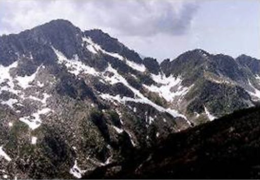
Input Image

Output Images for two different values of the parameter k


The forest created after a few iterations

Input Image
Output Images for two different values of the parameter k


The forest created after a few iterations

Input Image

Output Segmented Images


Input Image

Segmented Output Images

Input Image

Output Images for two different values of the parameter k


The forest created after a few iterations

Input Image (UMBC)

Segmented Output Images

Input Image

Segmented Output Image with k=0.001

Input Image

Segmented Output Image with k=0.001
Input Image

Segmented Output Image with k=0.001

Input Image (liver)

Segmented Output Images


Input Image

Segmented Output Images with different values of k


Input Image

Segmented Output Image

Input Image

Segmented Output Images for different k