
In the last few blog posts of this series discussed regression models at length. Fernando has built a multivariate regression model. The model takes the following shape:
price = -55089.98 + 87.34 engineSize + 60.93 horse power + 770.42 width
The model predicts or estimates price (target) as a function of engine size, horse power, and width (predictors).
Recall that multivariate regression model assumes independence between the independent predictors. It treats horsepower, engine size, and width as if they are not related.
In practice, variables are rarely independent.
What if there are relations between horsepower, engine size and width? Can these relationships be modeled?
This blog post will address this question. It will explain the concept of interactions.
The Concept:
The independence between predictors means that if one predictor changes, it has the impact on the target. This impact has no relation with existence or changes to other predictors. The relationship between the target and the predictors is additive and linear.
Let us take an example to illustrate it. Fernando’s equation is:
price = -55089.98 + 87.34 engine size + 60.93 horse power + 770.42 width
It is interpreted as a unit change to the engine size changes the price by $87.34.
This interpretation never takes into consideration that engine size may be related to the width of the car.
Can’t it be the case that wider the car, bigger the engine?
A third predictor captures the interaction between engine and width. This third predictor is called as the interaction term.
With the interaction term between engine size and the width, the regression model takes the following shape:
price = β0 + β1. engine size + β2. horse power + β3. width + β4. (engine size . width)
The part of the equation (β1. engine size + β3. width) is called as the main effect.
The term engine size x width is the interaction term.
How does this term capture the relation between engine size and width? We can rearrange this equation as:
price = β0 + (β1 + β4. width) engine size + β2. horse power + β3. width
Now, β4 can be interpreted as the impact on the engine size if the width is increased by 1 unit.
Model Building:
Fernando inputs these data into his statistical package. The package computes the parameters. The output is the following:
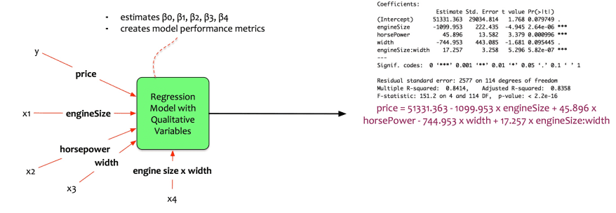
The equation becomes:
price = 51331.363–1099.953 x engineSize + 45.896 x horsePower — 744.953 x width + 17.257 x engineSize:width
price = 51331.363 — (1099.953–17.257 x width)engineSize + 45.896 x horsePower — 744.953 x width
Let us interpret the coefficients:
- The engine size, horse power and engine size: width (the interaction term) are significant.
- The width of the car is not significant.
- Increasing the engine size by 1 unit, reduces the price by $1099.953.
- Increasing the horse power by 1 unit, increases the price by $45.8.
- The interaction term is significant. This implies that the true relationship is not additive.
- Increasing the engine size by 1 unit, also increases the price by (1099.953–17.257 x width).
- The adjusted r-squared on test data is 0.8358 => the model explains 83.5% of variation.
Note that the width of the car is not significant. Then does it make sense to include it in the model?
Here comes a principle called as the hierarchical principle.
Hierarchical Principle: When interactions are included in the model, the main effects needs to be included in the model as well. The main effects needs to be included even if the individual variables are not significant in the model.
Fernando now runs the model and tests the model performance on test data.
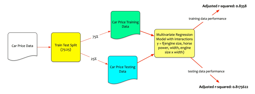
The model performs well on the testing data set. The adjusted r-squared on test data is 0.8175622 => the model explains 81.75% of variation on unseen data.
Fernando now has an optimal model to predict the car price and buy a car.
Limitations of Regression Models
Regression models are workhorse of data science. It is an amazing tool in a data scientist’s toolkit. When employed effectively, they are amazing at solving a lot of real life data science problems. Yet, they do have their limitations. Three limitations of regression models are explained briefly:
Non-linear relationships:
Linear regression models assume linearity between variables. If the relationship is not linear then the linear regression models may not perform as expected.
Practical Tip: Use transformations like log to transform a non-linear relationship to a linear relationship
Multi-Collinearity:
Collinearity refers to a situation where two predictor variables are correlated with each other. When there a lot of predictors and these predictors are correlated to each other, it is called as multi-collinearity. If the predictors are correlated with each other then the impact of a specific predictor on the target is difficult to be isolated.
Practical Tip: Make the model simpler by choosing predictors carefully. Limit choosing too many correlated predictors. Alternately, use techniques like principal components that create new uncorrelated variables.
Impact of outliers:
An Outlier is a point which is far from the value predicted by the model. If there are outliers in the target variable, the model is stretched to accommodate them. Too much model adjustment is done for a few outlier points. This makes the model skew towards the outliers. It doesn’t do any good in fitting the model for the majority.
Practical Tip: Remove the outlier points for modeling. If there are too many outliers in the target, there may be a need for multiple models.
Conclusion:
It has been quite a journey. In the last few blog posts, simple linear regression model was explained. Then we dabbled in multivariate regression models. Model selection methods were discussed. Treating qualitative variables and interaction were discussed as well.
In the next post of this series, we will discuss another type of supervised learning model: Classification.
Originally published at datascientia.blog