The covariance matrix has many interesting properties, and it can be found in mixture models, component analysis, Kalman filters, and more. Developing an intuition for how the covariance matrix operates is useful in understanding its practical implications. This article will focus on a few important properties, associated proofs, and then some interesting practical applications, i.e., extracting transformed polygons from a Gaussian mixture’s covariance matrix.

I have often found that research papers do not specify the matrices’ shapes when writing formulas. I have included this and other essential information to help data scientists code their own algorithms.

Sub-Covariance Matrices

The covariance matrix can be decomposed into multiple unique (2×2) covariance matrices. The number of unique sub-covariance matrices is equal to the number of elements in the lower half of the matrix, excluding the main diagonal. A (DxD) covariance matrices will have D*(D+1)/2 -D unique sub-covariance matrices. For example, a three dimensional covariance matrix is shown in equation (0).

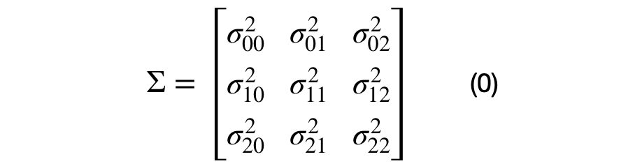
It can be seen that each element in the covariance matrix is represented by the covariance between each (i,j) dimension pair. Equation (1), shows the decomposition of a (DxD) into multiple (2×2) covariance matrices. For the (3×3) dimensional case, there will be 3*4/2–3, or 3, unique sub-covariance matrices.

Note that generating random sub-covariance matrices might not result in a valid covariance matrix. The covariance matrix must be positive semi-definite and the variance for each dimension the sub-covariance matrix must the same as the variance across the diagonal of the covariance matrix.

Positive Semi-Definite Property

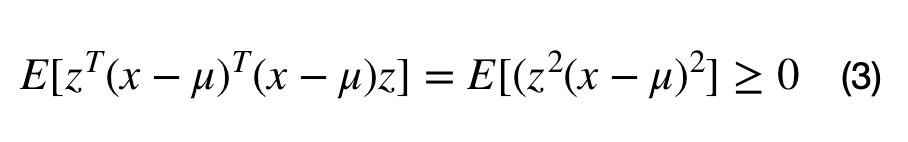
One of the covariance matrix’s properties is that it must be a positive semi-definite matrix. What positive definite means and why the covariance matrix is always positive semi-definite merits a separate article. In short, a matrix, M, is positive semi-definite if the operation shown in equation (2) results in a values which are greater than or equal to zero.

M is a real valued DxD matrix and z is an Dx1 vector. Note: the result of these operations result in a 1×1 matrix.

A covariance matrix, M, can be constructed from the data with the following operation, where the M = E[(x-mu).T*(x-mu)]. Inserting M into equation (2) lead to equation (3). It can be seen that any matrix that can be written in the form M.T*M is positive semi-definite. This full proof can be found here.

Note that the covariance matrix does not always describe the covariation between a dataset’s dimensions. For example, the covariance matrix can be used to describe the shape of a multivariate normal cluster, for Gaussian mixture models.

Geometric Implications

Another way to think about the covariance matrix is geometrically. Essentially, the covariance matrix represents the direction and scale for how the data is spread. To understand this perspective, it will be necessary to understand eigenvalues and eigenvectors.

Equation (4) shows the definition of an eigenvector and its associated eigenvalue. The next statement is important in understanding eigenvectors and eigenvalues. Z is an eigenvector of M if the matrix multiplication M*z results in the same vector, z, scaled by some value, lambda. In other words, we can think of the matrix M as a transformation matrix that does not change the direction of z, or z is a basis vector of matrix M.

Lambda is the eigenvalue (1×1) scalar, z is the eigenvector (Dx1) matrix, and M is the (DxD) covariance matrix. A positive semi-definite (DxD) covariance matrix will have D eigenvalue and (DxD) eigenvectors. The first eigenvector is always in the direction of highest spread of data, all eigenvectors are orthogonal to each other, and all eigenvectors are normalized, i.e. they have values between 0 and 1. Equation (5) shows the vectorized relationship between the covariance matrix, eigenvectors, and eigenvalues.

S is the (DxD) diagonal scaling matrix, where the diagonal values correspond to the eigenvalue and which represent the variance of each eigenvector. R is the (DxD) rotation matrix that represents the direction of each eigenvalue.

The eigenvector and eigenvalue matrices are represented, in the equations above, for a unique (i,j) sub-covariance matrix. The sub-covariance matrix’s eigenvectors, shown in equation (6), across each columns has one parameter, theta, that controls the amount of rotation between each (i,j) dimension pair. The covariance matrix’s eigenvalues are across the diagonal elements of equation (7) and represent the variance of each dimension. It has D parameters that control the scale of each eigenvector.

The Covariance Matrix Transformation

A (2×2) covariance matrix can transform a (2×1) vector by applying the associated scale and rotation matrix. The scale matrix must be applied before the rotation matrix as shown in equation (8).

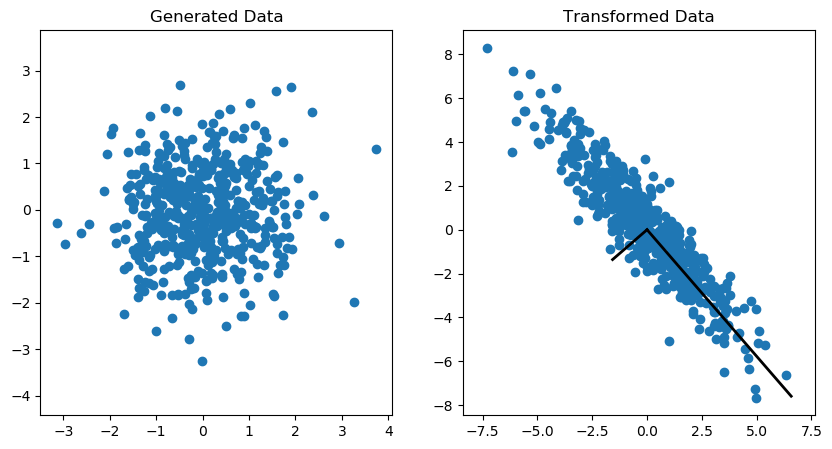
The vectorized covariance matrix transformation for a (Nx2) matrix, X, is shown in equation (9). The matrix, X, must centered at (0,0) in order for the vector to be rotated around the origin properly. If this matrix X is not centered, the data points will not be rotated around the origin.

An example of the covariance transformation on an (Nx2) matrix is shown in the Figure 1. More information on how to generate this plot can be found here.

Please see this link to see how these properties can be used to draw Gaussian mixture contours and create non-Gaussian, polygon, mixture models.

Originally posted by Rohan Kotwani