Comparing Spectral partitioning / clustering (with Normalized Graph Laplacian) with KMeans Clustering in R

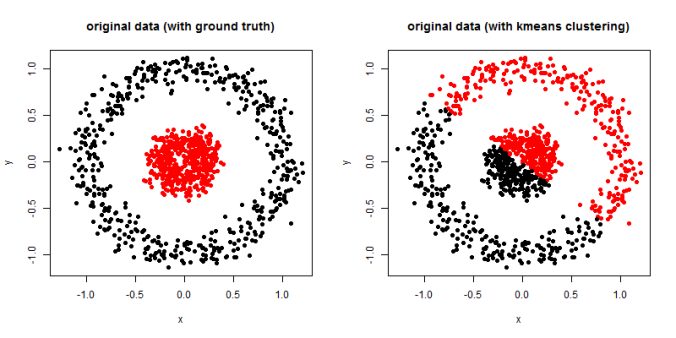
In this article, the clustering output results using Spectral clustering (with normalized Laplacian) are going to be compared with taht obtained using KMeans clustering on a few shape datasets. 

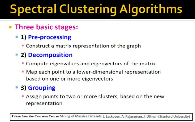
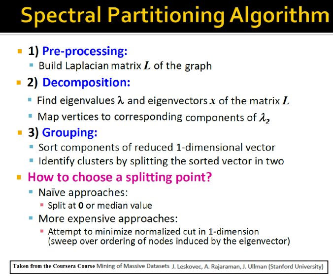
The following couple of slides taken from the Coursera Course: Mining Massive Datasets by Stanford University 
describe the basic concepts behind the spectral clustering and the spectral partitioning algorithms.

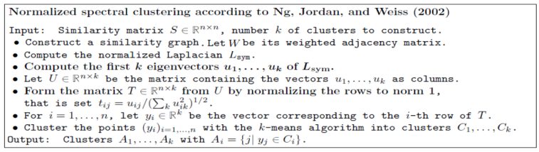
1. The spectral clustering algorithm has many variants. In this article, the following algorithm (by Ng. et al) is going to be used for the implementation of spectral clustering (with normalized Laplacian).

   

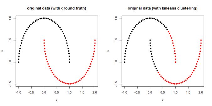
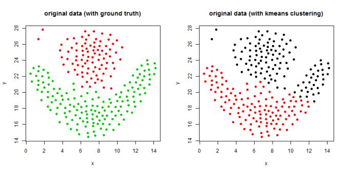
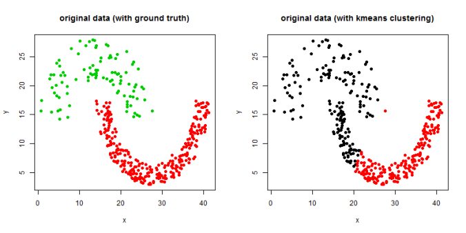
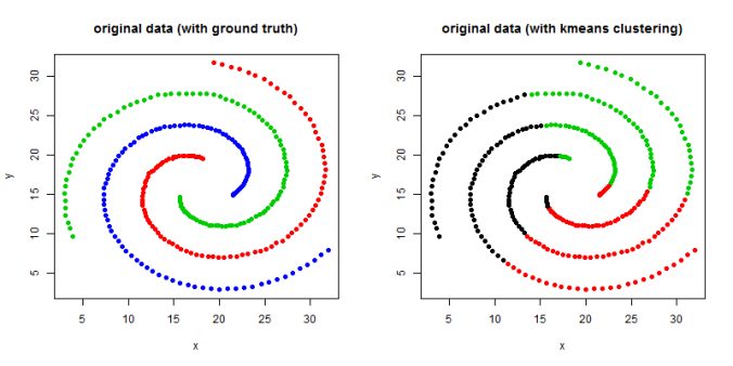
2. The following figures / animations show the spectral clustering results with different Gaussian similarity kernel bandwidth parameter values on different shape datasets and also the comparison with the results obtained using the KMeans counterpart.|

   
    />
   

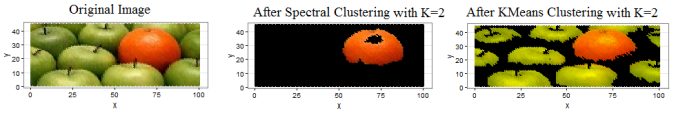
3. Finally, both KMeans and Spectral clustering (with bandwidth=0.1) algorithms are applied on the following apples and oranges image to segment the image into 2 clusters. As can be seen from the next figure, the spectral clustering (by clustering the first two dominant eigenvectors of the Normalized Laplacian) could separate out the orange from the apples, while the simple KMeans on the RGB channels could not.

   

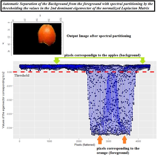
4. The following simpler spectral partitioning approach (thresholding on the second dominant eigenvector) can also be applied for automatic separation of the foreground from the background.

   

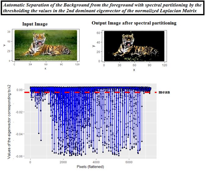
The following figure shows the result of spectral partitioning for automatic separation of foreground from the background on yet another image.