
Learn about CART in this guest post by Jillur Quddus, a lead technical architect, polyglot software engineer and data scientist with over 10 years of hands-on experience in architecting and engineering distributed, scalable, high-performance, and secure solutions used to combat serious organized crime, cybercrime, and fraud.
Although both linear regression models allow and logistic regression models allow us to predict a categorical outcome, both of these models assume a linear relationship between variables. Classification and Regression Trees (CART) overcome this problem by generating Decision Trees. These decision trees can then be traversed to come to a final decision, where the outcome can either be numerical (regression trees) or categorical (classification trees). A simple classification tree used by a mortgage lender is illustrated in the following diagram:
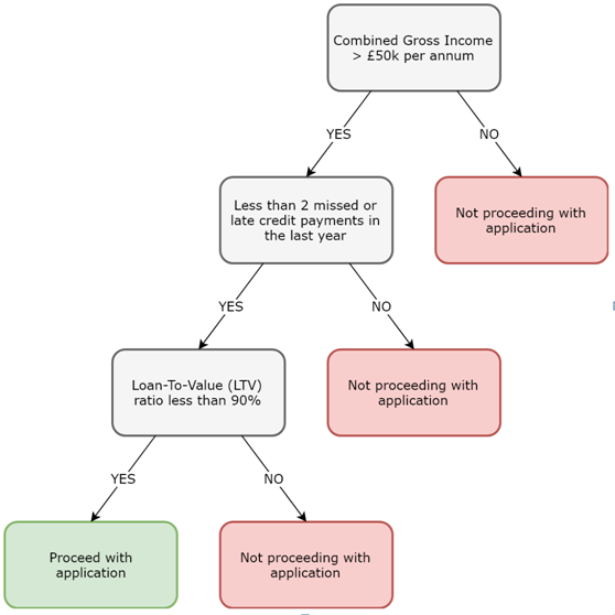
When traversing decision trees, start at the top. Thereafter, traverse left for yes, or positive responses, and traverse right for no, or negative responses. Once you reach the end of a branch, the leaf nodes describe the final outcome.
Case study – predicting political affiliation
For our next use case, we will use congressional voting records from the US House of Representatives to build a classification tree in order to predict whether a given congressman or woman is a Republican or a Democrat.
Note :
The specific congressional voting dataset that we will use can be availed from UCI’s machine learning repository at https://archive.ics.uci.edu/ml/datasets/congressional+voting+records. It has been cited by Dua, D., and KarraTaniskidou, E. (2017). UCI Machine Learning Repository [http://archive.ics.uci.edu/ml]. Irvine, CA: University of California, School of Information and Computer Science.
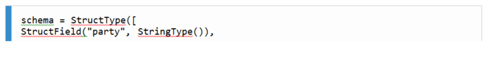
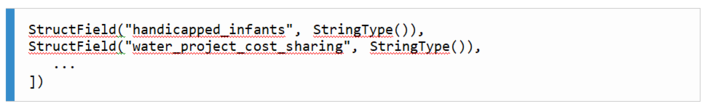
If you open congressional-voting-data/house-votes-84.data in any text editor of your chice, you will find 435 congressional voting records, of which 267 belong to Democrats and 168 belong to Republicans. The first column contains the label string, in other words, Democrat or Republican, and the subsequent columns indicate how the congressman or woman in question voted on particular key issues at the time (y = for, n = against, ? = neither for nor against), such as an anti-satellite weapons test ban and a reduction in funding to a synthetic fuels corporation. Let’s now develop a classification tree in order to predict the political affiliation of a given congressman or woman based on their voting records:
Note :
The following sub-sections describe each of the pertinent cells in the corresponding Jupyter Notebook for this use case, entitled chp04-04-classification-regression-trees.ipynb, and which may be found at https://github.com/PacktPublishing/Machine-Learning-with-Apache-Spa…. Note that for the sake of brevity, we will skip those cells that perform the same functions as seen previously.
- Since our raw data file has no header row, we need to explicitly define its schema before we can load it into a Spark DataFrame, as follows:
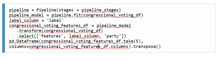
2. Since all of our columns, both the label and all the independent variables, are string-based data types, we need to apply a StringIndexer to them (as we did when developing our logistic regression model) in order to identify and index all possible categories for each column before generating numerical feature vectors. However, since we have multiple columns that we need to index, it is more efficient to build apipeline. A pipeline is a list of data and/or machine learning transformation stages to be applied to a Spark DataFrame. In our case, each stage in our pipeline will be the indexing of a different column as follows:
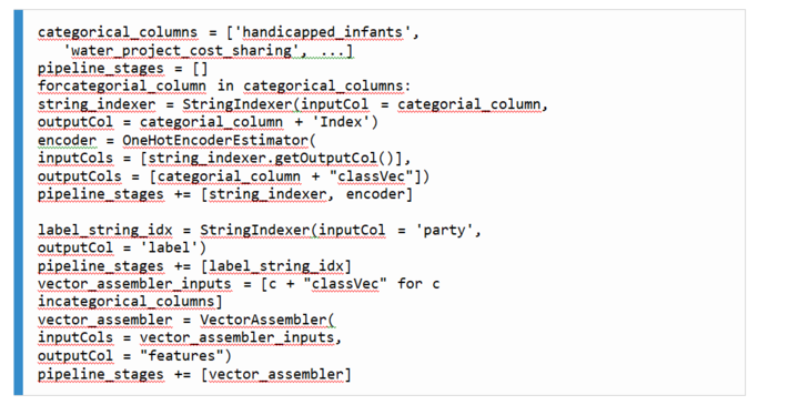
3. Next, we instantiate our pipeline by passing to it the list of stages that we generated in the previous cell. We then execute our pipeline on the raw Spark DataFrame using the fit() method, before proceeding to generate our numerical feature vectors using VectorAssembler as before:
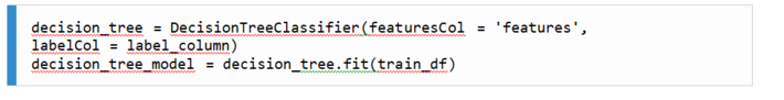
 4. We are now ready to train our classification tree! To achieve this, we can use MLlib’s DecisionTreeClassifier estimator to train a decision tree on our training dataset as follows:
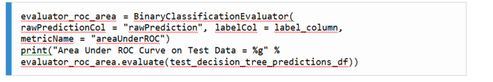
5. After training our classification tree, we will evaluate its performance on the test DataFrame. As with logistic regression, we can use the AUC metric as a measure of the proportion of time that the model predicts correctly. In our case, our model has an AUC metric of 0.91, which is very high:
6. Ideally, we would like to visualize our classification tree. Unfortunately, there is not yet any direct method in which to render a Spark decision tree without using third-party tools such as https://github.com/julioasotodv/spark-tree-plotting. However, we can render a text-based decision tree by invoking the toDebugString method on our trained classification tree model, as follows:

With an AUC value of 0.91, we can say that our classification tree model performs very well on the test data and is very good at predicting the political affiliation of congressmen and women based on their voting records. In fact, it classifies correctly 91% of the time across all threshold values!
Note that a CART model also generates probabilities, just like a logistic regression model. Therefore, we use a threshold value (default 0.5) in order to convert these probabilities into decisions, or classifications as in our example. There is, however, an added layer of complexity when it comes to training CART models—how do we control the number of splits in our decision tree?
One method is to set a lower limit for the number of training data points to put into each subset or bucket. In MLlib, this value is tuneable, via the minInstancesPerNode parameter, which is accessible when training our DecisionTreeClassifier. The smaller this value, the more splits that will be generated.
However, if it is too small, then overfitting will occur. Conversely, if it is too large, then our CART model will be too simple with a low level of accuracy. We will discuss how to select an appropriate value during our introduction to random forests next. Note that MLlib also exposes other configurable parameters, including maxDepth (the maximum depth of the tree) and maxBins, but note that the larger a tree becomes in terms of splits and depth, the more computationally expensive it is to compute and traverse. To learn more about the tuneable parameters available to a DecisionTreeClassifier, please visit https://spark.apache.org/docs/latest/ml-classification-regression.html.
Random forests
One method of improving the accuracy of CART models is to build multiple decision trees, not just the one. In random forests, we do just that—a large number of CART trees are generated and thereafter, each tree in the forest votes on the outcome, with the majority outcome taken as the final prediction.
To generate a random forest, a process known as bootstrapping is employed whereby the training data for each tree making up the forest is selected randomly with replacement. Therefore, each individual tree will be trained using a different subset of independent variables and, hence, different training data.
K-Fold cross validation
Let’s now return to the challenge of choosing an appropriate lower-bound bucket size for an individual decision tree. This challenge is particularly pertinent when training a random forest since the computational complexity increases with the number of trees in the forest. To choose an appropriate minimum bucket size, we can employ a process known as K-Fold cross validation, the steps of which are as follows:
- Split a given training dataset into K subsets or “folds” of equal size.
- (K – 1) folds are then used to train the model, with the remaining fold, called the validation set, used to test the model and make predictions for each lower-bound bucket size value under consideration.
- This process is then repeated for all possible training and test fold combinations, resulting in the generation of multiple trained models that have been tested on each fold for every lower-bound bucket size value under consideration.
- For each lower-bound bucket size value under consideration, and for each fold, calculate the accuracy of the model on that combination pair.
- Finally, for each fold, plot the calculated accuracy of the model against each lower-bound bucket size value, as illustrated in Figure 4.8:
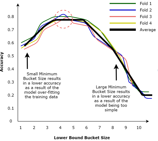
As illustrated in the above graph, choosing a small lower-bound bucket size value results in lower accuracy as a result of the model overfitting the training data. Conversely, choosing a large lower-bound bucket size value also results in lower accuracy as the model is too simple. Therefore, in our case, we would choose a lower-bound bucket size value of around 4 or 5, since the average accuracy of the model seems to be maximized in that region (as illustrated by the dashed circle in the above diagram).
Returning to our Jupyter Notebook, chp04-04-classification-regression-trees.ipynb, let’s now train a random forest model using the same congressional voting dataset to see whether it results in a better performing model compared to our single classification tree that we developed previously:
- To build a random forest, we can use MLlib’s RandomForestClassifier estimator to train a random forest on our training dataset, specifying the minimum number of instances each child must have after a split via the minInstancesPerNode parameter, as follows:

2. We can now evaluate the performance of our trained random forest model on our test dataset by computing the AUC metric using the same BinaryClassificationEvaluator as follows:
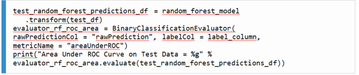
Our trained random forest model has an AUC value of 0.97, meaning that it is more accurate in predicting political affiliation based on historical voting records than our single classification tree!
If you found this article helpful and would like to learn more about machine learning, you must explore Machine Learning with Apache Spark Quick Start Guide. Written by Jillur Quddus, Machine Learning with Apache Spark Quick Start Guide combines the latest scalable technologies with advanced analytical algorithms using real-world use-cases in order to derive actionable insights from Big Data in real-time.