
As per Wikipedia, Price Elasticity of Demand (PED or ED or PE) is a measure used in economics to show the responsiveness, or change, of the quantity demanded of a good or service to a change in its price when nothing but the price changes. In more precise business terms, it helps in finding those products which have their sales more/less susceptible to price changes. As we know, the demand is inversely proportional to price, it is quite imperative to know this information for optimising sales and margins.
Without going much into literature of Price Elasticity (PE), I shall explain how I implemented ‘no-code-analytics’ through KNIME to get the PE values from real sales and price data. I also calculated Cross Price Elasticity (CPE) since I had competitor prices at my disposal too. I shall be highlighting all the modules that I used along with the respective input-output.
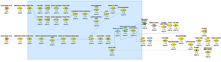
As in any analytics project, here also the major weight lifting is data engineering – getting the data in shape for the final model to run. I started with the two Excel Reader (1) modules to ingest price and sales data. The first thing I did was drop couple of unnecessary columns like county, company, model name (I will use part numbers to identify a product), short description, list price, discount etc. using the module Column Filter (2). The very first column I engineered was date column, to remove time stamp and filter just date using the Date & Time to String (3) module. Now I removed unnecessary rows with junk values using the Row Filter (4.1) module. If a dataset requires special treatment, you can filter those rows and then append to the main data using Concatenate (4.2) module post processing. Now comes the interesting part, converting the long format data to wide. I need only one row for all the prices (across competing retailers) a product had on a particular day. Hence, as an output, I will have all the retailers in the data in respective columns, with price on that particular day as value. For this I used Pivoting (5) module with part number & date as grouping columns, retailer will go into columns and price would be the value selected. It doesn’t allow you to aggregate multiple values and hence you have to use the Column Aggregator (6) module. There is flexibility of selecting the aggregation mode. In my case, I selected the minimum value so that I can capture the most competitive seller price on a marketplace website. Now, it is time to join price data with sales data (which was being processed in parallel). The join was achieved using Joiner (7) module. You can select the join mode (inner, outer etc.), which columns to be used to join and which columns are to be kept in the final output. If you want to do any kind of manipulation on date e.g. extracting day/year, changing the format, getting the week number etc., you can do it by modules Extract Date & Time Fields (8.1), Number To String (8.2) and String Manipulation (8.3).
Now we try to implement a regression model on every sales X price combination for a part number across the time period. So, we have to loop on every part number and run a regression model for each part number. I must say, doing this is much easier in an R or Python compared to KNIME. Start with a Group Loop Start (9.1) module. Then comes the Linear regression Learner (9.2) to run the model on single part number. But since it doesn’t provide an R2 value, you would have to take a circuitous route involving Regression Predictor (9.3) with outputs from Loop (data) & Regression learner (equation) as input. Numeric Scorer (9.4) will provide the R2 value, Constant Value Column (9.5) shall add the loop iteration identifier column to data to later join with the coefficients coming from Regression Learner (9.2). Post joining the Coefficients and R2 values using Joiner (9.8), loop can be closed using Loop End (9.9). In between, there are also two important stages – RowID (9.6): helps in identifying the R2 value among multiple values and then Row Filter (9.7): helps in keeping only R2 value and removing rest of statistics.
Use a Joiner (10) to combine sales, prices, coefficients and R2 values in one table. Now, we can now use the module Math Formula Multi Column (11) to apply the formulas:
Sale = Intercept + A*Own Price + B*Competitor Price
Own Price Elasticity = A* (average Own price/average Own sales)
Cross Price Elasticity = B*(average Competitor Price/average Own sales)
Fig 1: The arrangement of modules to run regression in loop and get coefficients/R2 values
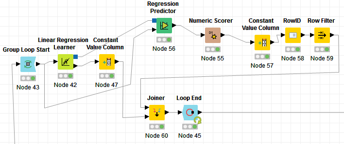
Fig 2: The output of Numeric Scorer
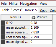
Fig 3: The output from Constant Value Column (9.5)
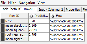
Fig 4: The output from RowID (9.6)
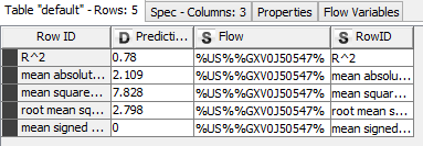
Fig 5: Complete Flow