
Face recognition is a combination of two major operations: face detection followed by Face classification. In this tutorial, we will look into a specific use case of object detection – face recognition.
The pipeline for the concerned project is as follows:
- Face detection: Look at an image and find all the possible faces in it
- Face extraction: Focus on each face image and understand it, for example, if it is turned sideways or badly lit
- Feature extraction: Extract unique features from the faces using convolutional neural networks (CNNs)
- Classifier training: Finally, compare the unique features of that face to all the people already known, to determine the person’s name
We will learn the main ideas behind each step, and how to raise our own facial recognition system in Python using the following deep-learning technologies:
- dlib(http://dlib.net/): Provides a library that can be used for facial detection and alignment.
- OpenFace(https://cmusatyalab.github.io/openface/): A deep-learning facial recognition model, developed by Brandon Amos et al (http://bamos.github.io/). It is able to run on real-time mobile devices as well.
- FaceNet(https://arxiv.org/abs/1503.03832): A CNN architecture that is used for feature extraction. For a loss function, FaceNet uses triplet loss. Triplet loss relies on minimizing the distance from positive examples while maximizing the distance from negative examples.
Setting up Environment
Since setup can get very complicated and takes a long time, we will be building a Docker image that contains all the dependencies, including dlib, OpenFace, and FaceNet.
Getting the code
Fetch the code that we will use to build face recognition from the repository:
git clone https://github.com/PacktPublishing/Python-Deep-Learning-Projects cd Chapter10/
Building the Docker Image
Docker is a container platform that simplifies deployment. It solves the problem of installing software dependencies onto different server environments. If you are new to Docker, you can read more at https://www.docker.com/.
To install Docker on Linux machines, run the following command:
curl https://get.docker.com | sh
For other systems such as macOS and Windows, visit https://docs.docker.com/install/.You can skip this step if you already have Docker installed.
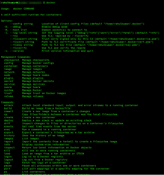
Once Docker is installed, you should be able to use the docker command in the Terminal, as follows:
Now, we will create a docker file that will install all the dependencies, including OpenCV, dlib, and TensorFlow.
#Dockerfile for our env setup
FROM tensorflow/tensorflow:latest
RUN apt-get update -y --fix-missing
RUN apt-get install -y ffmpeg
RUN apt-get install -y build-essential cmake pkg-config \ libjpeg8-dev libtiff5-dev libjasper-dev libpng12-dev \ libavcodec-dev libavformat-dev libswscale-dev libv4l-dev \ libxvidcore-dev libx264-dev \ libgtk-3-dev \ libatlas-base-dev gfortran \ libboost-all-dev \ python3 python3-dev python3-numpy
RUN apt-get install -y wget vim python3-tk python3-pip
WORKDIR /RUN wget -O opencv.zip https://github.com/Itseez/opencv/archive/3.2.0.zip \ && unzip opencv.zip \ && wget -O opencv_contrib.zip
https://github.com/Itseez/opencv_contrib/archive/3.2.0.zip \ && unzip opencv_contrib.zip
# install opencv3.2
RUN cd /opencv-3.2.0/ \
&& mkdir build \
&& cd build \
&& cmake -D CMAKE_BUILD_TYPE=RELEASE \
-D INSTALL_C_EXAMPLES=OFF \
-D INSTALL_PYTHON_EXAMPLES=ON \
-D OPENCV_EXTRA_MODULES_PATH=/opencv_contrib-3.2.0/modules \
-D BUILD_EXAMPLES=OFF \
-D BUILD_opencv_python2=OFF \
-D BUILD_NEW_PYTHON_SUPPORT=ON \
-D CMAKE_INSTALL_PREFIX=$(python3 -c "import sys; print(sys.prefix)") \
-D PYTHON_EXECUTABLE=$(which python3) \
-D WITH_FFMPEG=1 \
-D WITH_CUDA=0 \ .. \
&& make -j8 \
&& make install \
&& ldconfig \
&& rm /opencv.zip \
&& rm /opencv_contrib.zip # Install dlib 19.4RUN wget -O dlib-19.4.tar.bz2 http://dlib.net/files/dlib-19.4.tar.bz2 \
&& tar -vxjf dlib-19.4.tar.bz2 RUN cd dlib-19.4 \
&& cd examples \
&& mkdir build \
&& cd build \
&& cmake .. \
&& cmake --build . --config Release \
&& cd /dlib-19.4 \
&& pip3 install setuptools \
&& python3 setup.py install \
&& cd $WORKDIR \
&& rm /dlib-19.4.tar.bz2 ADD $PWD/requirements.txt /requirements.txtRUN pip3 install -r /requirements.txt CMD ["/bin/bash"]
Now execute the following command to build the image:
docker build -t hellorahulk/facerecognition -f Dockerfile
It will take approximately 20-30 minutes to install all the dependencies and build the Docker Image:

Downloading Pre-Trained Models
We will download a few more artifacts, which we will use and discuss in detail later in this tutorial. Download Dlib’s face landmark predictor, using the following commands:
curl -O http://dlib.net/
files/shape_predictor_68_face_landmarks.dat.bz2
bzip2 -d shape_predictor_68_face_landmarks.dat.bz2
cp shape_predictor_68_face_landmarks.dat facenet/
Download the pre-trained inception model:
curl -L -O https://www.dropbox.com/s/hb75vuur8olyrtw/Resnet-185253.pbcp Resnet-185253.pb pre-model/
Once we have all the components ready, the folder structure should look roughly as follows:
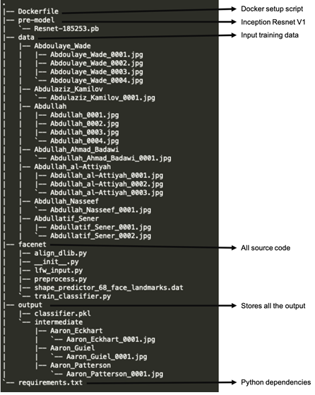
Folder Structure of the Code
Make sure that you keep the images of the person you want to train the model within the /data folder, and name the folder as /data/<class_name>/<class_name>_000<count>.jpg.
The /output folder will contain the trained SVM classifier and all pre-processed images inside a subfolder /intermediate, using the same folder nomenclature as in the /data folder.
For better performance in terms of accuracy, keeping more than five samples of images for each class is suggested. This helps the model to converge faster and generalize better.
Building the Pipeline
Facial recognition is a biometric solution that measures the unique characteristics of faces. To perform facial recognition, you’ll need a way to uniquely represent a face. The main idea behind any face recognition system is to break the face down into unique features, and then use those features to represent identity.
Building a robust pipeline for feature extraction is very important, as it will directly affect the performance and accuracy of our system.
To build the face recognition pipeline, we will devise the following flow (represented by orange blocks in the diagram):
- Pre-processing: Finding all the faces, fixing the orientation of the faces
- Feature extraction: Extracting unique features from the processed faces
- Classifier training: Training the SVM classifier with 128-dimensional features

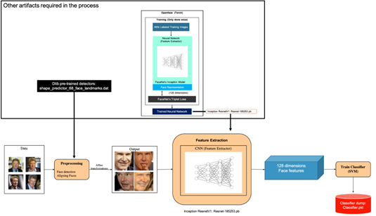
This image illustrates the end to end flow for face recognition pipeline. We will look into each of the steps, and build our world-class face recognition system.
Pre-processing of Images
The first step in our pipeline is face detection. We will then align the faces, extract features, and then finalize our pre-processing on Docker.
Face detection
Obviously, it’s very important to first locate the faces in the given photograph so that they can be fed into the later part of the pipeline. There are many ways to detect faces, such as detecting skin textures, oval/round shape detection, and other statistical methods. We’re going to use a method called HOG.
HOG is a feature descriptor that represents the distribution (histograms) of directions of gradients (oriented gradients), which are used as features. Gradients (x and y derivatives) of an image are useful because the magnitude of gradients is large around edges and corners (regions of abrupt intensity changes), which are excellent features in a given image.
To find faces in an image, we’ll convert the image into greyscale. Then we’ll look at every single pixel in our image, one at a time, and try to extract the orientation of the pixels using the HOG detector. We’ll be using dlib.get_frontal_face_detector() to create our face detector.
The following small snippet demonstrates the HOG-based face detector being used in the implementation:
import sysimport dlibfrom skimage import io
# Create a HOG face detector using the built-in dlib classface_detector = dlib.get_frontal_face_detector()
# Load the image into an arrayfile_name = 'sample_face_image.jpeg'image = io.imread(file_name)
# Run the HOG face detector on the image data.
# The result will be the bounding boxes of the faces in our image.detected_faces = face_detector(image, 1) print("Found {} faces.".format(len(detected_faces)))
# Loop through each face we found in the imagefor i, face_rect in enumerate(detected_faces):
# Detected faces are returned as an object with the coordinates
# of the top, left, right and bottom edges print("- Face #{} found at Left: {} Top: {} Right: {} Bottom: {}".format(i+1, face_rect.left(), face_rect.top(), face_rect.right(), face_rect.bottom()))
The output is as follows:
Found 1 faces.
-Face #1 found at Left: 365 Top: 365 Right: 588 Bottom: 588
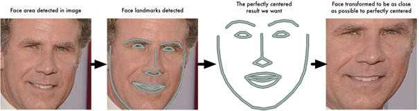
Aligning Faces
Once we know the region in which the face is located, we can perform various kinds of isolation techniques to extract the face from the overall image.
One challenge to deal with is that faces in images may be turned in different directions, making them look different to the machine.
To solve this issue, we will warp each image so that the eyes and lips are always in the sample place in the provided images. This will make it a lot easier for us to compare faces in the next steps. To do so, we are going to use an algorithm called face landmark estimation.
The basic idea is to come up with 68 specific points (called landmarks) that exist on every face—the top of the chin, the outside edge of each eye, the inner edge of each eyebrow, and so on. Then we will train a machine-learning algorithm to be able to find these 68 specific points on any face.
The 68 landmarks we will locate on every face are shown in the following diagram:
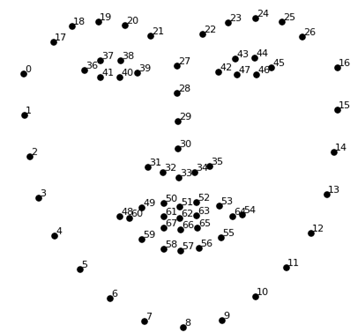
This image was created by Brandon Amos (http://bamos.github.io/), who works on OpenFace (https://github.com/cmusatyalab/openface).
Here is a small snippet demonstrating how to use face landmarks, which we downloaded in the Setup environment section:
import sys
import dlib
import cv2
import openface
predictor_model = "shape_predictor_68_face_landmarks.dat"
# Create a HOG face detector , Shape Predictor and Aligner
face_detector = dlib.get_frontal_face_detector()
face_pose_predictor = dlib.shape_predictor(predictor_model)
face_aligner = openface.AlignDlib(predictor_model)
# Take the image file name from the command line
file_name = 'sample_face_image.jpeg'
# Load the image
image = cv2.imread(file_name)
# Run the HOG face detector on the image data
detected_faces = face_detector(image, 1) print("Found {} faces.".format(len(detected_faces))
# Loop through each face we found in the image
for i, face_rect in enumerate(detected_faces):
# Detected faces are returned as an object with the coordinates
# of the top, left, right and bottom edges
print("- Face #{} found at Left: {} Top: {} Right: {} Bottom: {}".format(i, face_rect.left(), face_rect.top(), face_rect.right(), face_rect.bottom()))
# Get the the face's pose
pose_landmarks = face_pose_predictor(image, face_rect)
# Use openface to calculate and perform the face alignment
alignedFace = face_aligner.align(534, image, face_rect, landmarkIndices=openface.AlignDlib.OUTER_EYES_AND_NOSE)
# Save the aligned image to a file
cv2.imwrite("aligned_face_{}.jpg".format(i), alignedFace)
Using this, we can perform various basic image transformations such as rotation and scaling while preserving parallel lines. These are also known as affine transformations (https://en.wikipedia.org/wiki/Affine_transformation).
The output is as follows:
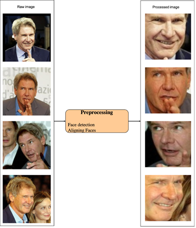
With segmentation, we solved finding the largest face in an image, and with alignment, we standardized the input image to be in the centre based on the location of eyes and bottom lip.
Here is a sample from our dataset, showing the raw image and processed image:
Feature Extraction
Now that we’ve segmented and aligned the data, we’ll generate vector embeddings of each identity. These embeddings can then be used as input to classification, regression, or clustering task.
This process of training CNN to output face embeddings requires a lot of data and computer power. However, once the network has been trained, it can generate measurements for any face, even ones it has never seen before! So this step only needs to be done once.
For convenience, we have provided a model that has been pre-trained on Inception-Resnet-v1, which you can run over any face image to get the 128 dimension feature vectors. We downloaded this file in the Setup environment section, and it’s located in the /pre-model/Resnet-185253.pb directory.
If you want to try this step yourself, OpenFace provides a Lua script (https://github.com/cmusatyalab/openface/blob/master/batch-represent…) that will generate embeddings for all images in a folder and write them to a CSV file.
The code to create the embeddings for the input images can be found further after the paragraph.
In the process, we are loading trained components from the Resnet model such as embedding_layer, images_placeholder, and phase_train_placeholder, along with the images and the labels:
def _create_embeddings(embedding_layer, images, labels, images_placeholder, phase_train_placeholder, sess): """ Uses model to generate embeddings from :param images. :param embedding_layer: :param images: :param labels: :param images_placeholder: :param phase_train_placeholder: :param sess: :return: (tuple): image embeddings and labels """ emb_array = None label_array = None try: i = 0 while True: batch_images, batch_labels = sess.run([images, labels]) logger.info('Processing iteration {} batch of size: {}'.format(i, len(batch_labels))) emb = sess.run(embedding_layer, feed_dict={images_placeholder: batch_images, phase_train_placeholder: False}) emb_array = np.concatenate([emb_array, emb]) if emb_array is not None else emb label_array = np.concatenate([label_array, batch_labels]) if label_array is not None else batch_labels i += 1 except tf.errors.OutOfRangeError: pass return emb_array, label_array
Here is a quick view of the embedding creating process. We fed the image and the label data along with few components from the pre-trained model:
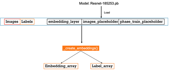
The output of the process will be a vector of 128 dimensions, representing the facial image.
Execution on Docker
We will implement pre-processing on our Docker image. We’ll mount the project directory as a volume inside the Docker container (using a -v flag), and run the pre-processing script on the input data. The results will be written to a directory specified with command-line arguments.
The align_dlib.py file is sourced from CMU. It provides methods for detecting a face in an image, finding facial landmarks, and aligning these landmarks:
docker run -v $PWD:/facerecognition \
-e PYTHONPATH=$PYTHONPATH:/facerecognition \
-it hellorahulk/facerecognition python3 /facerecognition/facenet/preprocess.py \
--input-dir /facerecognition/data \
--output-dir /facerecognition/output/intermediate \
--crop-dim 180
In the preceding command, we are setting the input data path using a –input-dir flag. This directory should contain the images that we want to process. We are also setting the output path using a –output-dir flag, which will store the segmented aligned images. We will be using these output images as input for training.
The –crop-dim flag is to define the output dimensions of the image. In this case, all images will be stored at 180 × 180. The outcome of this process will be a /intermediate folder being created inside the /output folder, containing all the pre-processed images.
Training the Classifier
First, we’ll load the segmented and aligned images from the input directory –input-dir flag. While training, we’ll apply to pre-process the image. This pre-processing will add random transformations to the image, creating more images to train on.
These images will be fed in a batch size of 128 into the pre-trained model. This model will return a 128-dimensional embedding for each image, returning a 128 x 128 matrix for each batch. After these embeddings are created, we’ll use them as feature inputs into a scikit-learn SVM classifier to train on each identity.
The following command will start the process, and train the classifier. The classifier will be dumped as a pickle file in the path defined in the –classifier-path argument:
docker run -v $PWD:/facerecognition \
-e PYTHONPATH=$PYTHONPATH:/facerecognition \
-it hellorahulk/facerecognition \python3 /facerecognition/facenet/train_classifier.py \
--input-dir /facerecognition/output/intermediate \
--model-path /facerecognition/pre-model/Resnet-185253.pb \
--classifier-path /facerecognition/output/classifier.pkl \
--num-threads 16 \
--num-epochs 25 \
--min-num-images-per-class 10 \
--is-train
- –num-threads: Modify according to the CPU/GPU config
- –num-epochs: Change according to your dataset
- –min-num-images-per-class: Change according to your dataset
- –is-train: Set the True flag for training
This process will take a while, depending on the number of images we are training on. Once the process is completed, we will find a classifier.pkl file inside the /output folder.
Now you can use the classifier.pkl file to make predictions, and deploy it on production.
Evaluation
We will evaluate the performance of the trained model by executing the following command:
docker run -v $PWD:/facerecognition \
-e PYTHONPATH=$PYTHONPATH:/facerecognition \
-it hellorahulk/facerecognition \python3 /facerecognition/facenet/train_classifier.py \
--input-dir /facerecognition/output/intermediate \
--model-path /facerecognition/pre-model/Resnet-185253.pb \
--classifier-path /facerecognition/output/classifier.pkl \
--num-threads 16 \
--num-epochs 2 \
--min-num-images-per-class 10 \
Once the execution is completed, we will see predictions with a confidence score, as shown in the following screenshot:
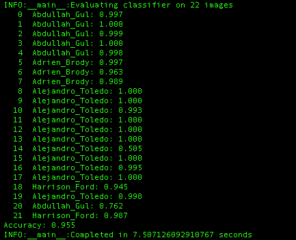
We can see that the model is able to predict with 99.5% accuracy. It is also relatively fast.
We have successfully completed a world-class facial recognition POC for our hypothetical high-performance data centre, utilizing deep learning technologies of OpenFace, Dlib, and FaceNet. This project is a great example of the power of deep learning to produce solutions that make a meaningful impact on the business operations of our clients.
If this tutorial kept you engaged and you wish to explore more, ‘Python: Beginner’s Guide to Artificial Intelligence’ could be the one you might find useful. This book will introduce to various machine learning and deep learning algorithms from scratch. Along with that, you’ll also be exposed to implementing them practically. Apart from that, you will learn to build accurate predictive models with TensorFlow, combined with other open-source Python libraries.