
1. Abstract
The objective of this paper is to present the process of building a Deep Learning Model for optimising the output for a Production Process from a Training sample using Weka Multilayer Perceptron. The scope is limited to implementation only and does not cover the theory behind Artificial Neural Networks. The Genetic Algorithm is specifically developed and adapted for the kind of data involved and is dealt with in detail
This work is the outcome of a comprehensive prototyping and proof-of-concept exercise conducted at Turing Point (http://www.turing-point.com/) a consulting company focused on providing genuine Enterprise Machine Learning solutions based on highly advanced techniques such as 3D discrete event simulation, deep learning and genetic algorithms.
2. Introduction
Predictive Analytics is the process of extracting information from the data for predicting future trends. There are a number of Machine Learning approaches available to model the behaviour.
Regression Techniques try to identify the underlying mathematical relationship between the dependent variables in data. Linear Regression, Logistic Regression, Quadratic Regression are some of the known Regression techniques.
Other Machine Learning techniques learn from training samples by emulating Human cognition. They are often employed in complex situations wherein the underlying mathematical relation is far too complex or hard to identify. Artificial Neural Networks or Multilayer Perceptron, Naïve Bayes Classifier, K Nearest Neighbour are some of the other known Machine Learning Techniques.
Deep Learning is a rapidly growing area of Machine Learning based on the knowledge of the human brain and development of statistics and applied maths over the past several decades. It focuses on algorithms that aim at extracting higher levels of abstractions in data using Artificial Neural Networks with multiple hidden layers.
3. Production Process
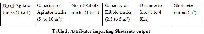
This section outlines the Production Process known as ‘Shotcrete (Concrete Spraying)’ for which an optimum solution is sought. This involves picking up the concrete mix from the plant by the agitator trucks. The concrete is mixed in the agitator tanks and transported to a drop hole of an underground work site. The dropped concrete are picked up by the Kibble trucks and transported to the application site where they are sprayed by the Shotcrete guns on the roadways being built. The objective is to maximise the daily Shotcrete Road Development volume (in m3) by identifying the right combination of the agitator trucks which can range from 1 to 4, the agitator tank capacities which can range from 5 to 10 m3, the number of Kibble trucks which can range from 1 to 5, the kibble tank capacities ranging from 2 to 5 m3 and the final parameter being the distance to application site which can range from 1 to 4 Kms.
4. Steps involved
The Model building process involves the following steps
- Gathering Training Sample Data
- Identifying the Deep Learning Model
- Training the Model
- Using the Genetic Algorithm to identify the combination of agitator and kibble trucks with their capacities and the distance to site for maximising the Shotcrete output.
4.1 Gathering Training Sample Data
The training sample should contain samples that would represent all possible variations in data. For example if the dataset contains just 2 inputs A and B, each of which taking a range of values say from 0 to 10000 units and assuming that both the A & B independently impact the Output. Then we need to have representative samples of variations in data as represented in Table 1
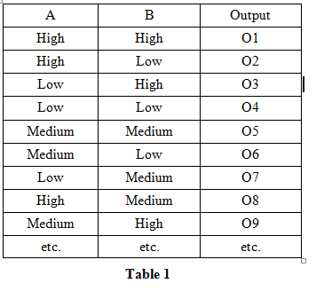
The Shotcrete spraying is concerned with the attributes in the first 5 columns for the output in column 6 of Table 2. The samples should capture variations in parameters so as to build a model that closely represents the way the 5 inputs affect the outputs. With this is view 182 samples were collected.
4.2 Identifying the Deep Learning Model
The Multilayer Perceptron of the Weka Machine Learning Tools from the University of Waikato, New Zealand is used for building the neural network model.
The model requires 5 inputs one for each of the attribute. There is one final output for Shotcrete Production output. In between these two, the number of hidden layers and the number of neurons in each of them will need to be decided. There is no definite rule for deciding this and experimentation is required. By default MLP (short for Multilayer Perceptron) creates one hidden layer. The number of neurons in this layer is the average of the number of inputs and output (hence 3 for the Shotcrete model).
A number of experiments were performed with multiple hidden layers. It was found that networks with 3 hidden layers (and hence a deep neural network) was able to perform much better in training and emulating the actual behaviour than the ones with 1 and 2 hidden layers respectively. The training aspect, the ability to reach global minima and the performance will be covered in the next section.
Figure 1, Figure 2 and Figure 3 cover some of the neural network architectures experimented with, having 1, 2 and 3 hidden layers respectively.
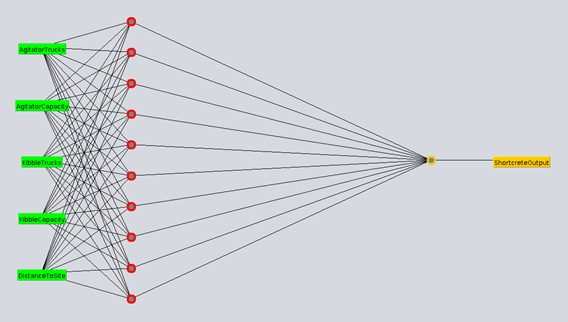
Figure 1 Neural Network with single layer of 10 neurons
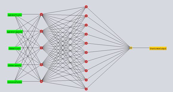
Figure 2 Neural Network with 2 hidden layers with 5 and 10 neurons respectively
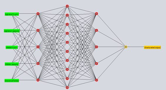 Figure 3 Neural Network with 3 hidden layers having 5,10 and 5 neurons respectively in each layer
4.3 Training Neural Networks
The training criterion is to reach global minima wherein the error on Epoch does not change significantly over several thousands of Epochs. To achieve this, the number of epochs was set at 50,000,000.
Learning rate and Momentum needed to be adjusted as well. If not, the errors were found to increase after to getting to the minima or oscillate around some value.
Weka Neural Networks use backpropagation algorithm. Without going into details of this algorithm (as it is beyond the scope of this paper) it is sufficient to state that there are two phases to each epoch:
- A forward pass through the network using the weights of the previous iteration (zero for the first epoch) is carried out and the output is computed. The error between the output and actual is used to calculate the gradient.
- The weight of each connection is adjusted and back propagated till the input layer using the following relationship
ΔWeach connection= -learning rate * gradient + momentum * ΔWeach connection computed during previous epoch
After some experimentation, training was found to be effective with the following parameters:
learning rate = 0.1
momentum = 0.1
The errors were computed for each of neural network architectures in Figure 1, Figure 2 and Figure 3 respectively.
For the single hidden network layer architecture described in Figure 1, the errors are as follows:
Mean absolute error 0.6399
Root mean squared error 0.8258
For the architecture having 2 hidden layers described in Figure 2, the errors are as follows:
Mean absolute error 0.4338
Root mean squared error 0.5739
Finally for the deep network architecture having 3 hidden layers described in Figure 3
Mean absolute error 0.082
Root mean squared error 0.1106
As can be seen above the deep architecture with 3 hidden layers yields the minimum error and hence has been chosen for predicting the Shotcrete output.
4.4 Searching for optimal combination of inputs using Genetic Algorithm
Having identified the model that would emulate the behaviour of Shotcrete Production process, the next goal is to identify the combination of Agitator trucks, Agitator capacity, Kibble trucks, Kibble capacity and the distance to site that would maximise the Shotcrete output. One way to do is to perform an exhaustive search of all possible combination of the inputs and use the neural network to predict the output values. This would require extensive computation and may not be practicable in situations involving a large number of parameters.
Genetic Algorithm provides good search heuristic that helps in narrowing down the search for optimal solutions. These algorithms are based on the theory of evolution of organisms, that survive the changing environment as described below:
Supposing there are 2 data points having attributes from A to J and A1 to J1 respectively that are used to produce outputs O and O1 respectively. Let it be assumed that the outputs O and O1 are reasonably high in “fitness” scores.
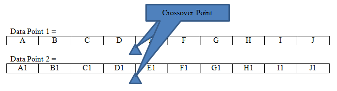
The “mating” of these 2 data points (aka Chromosomes) results in the children. A random crossover point between 1 and 10 (the total number of attributes in each data point) is generated. For the sake of this example in question let the cross over point be 4.
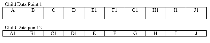
This can now generate 2 new data points by combining the attributes prior to the crossover point of one with the attributes after the crossover point of the other.
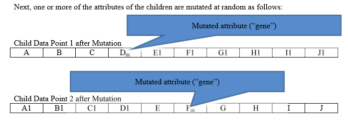
The idea is that the children generated from the mating of chromosomes with high fitness scores are highly likely to be good performers and thereby reducing the search for top performers. The fitness of the children data points generated this way can sometimes surpass the parent chromosomes as well. The process of creating new generations of candidates is continued till a threshold level of generations is reached wherein no further improvement in the ‘fittest’ can be achieved.
The search used for optimising Shotcrete output is covered in the following flowchart
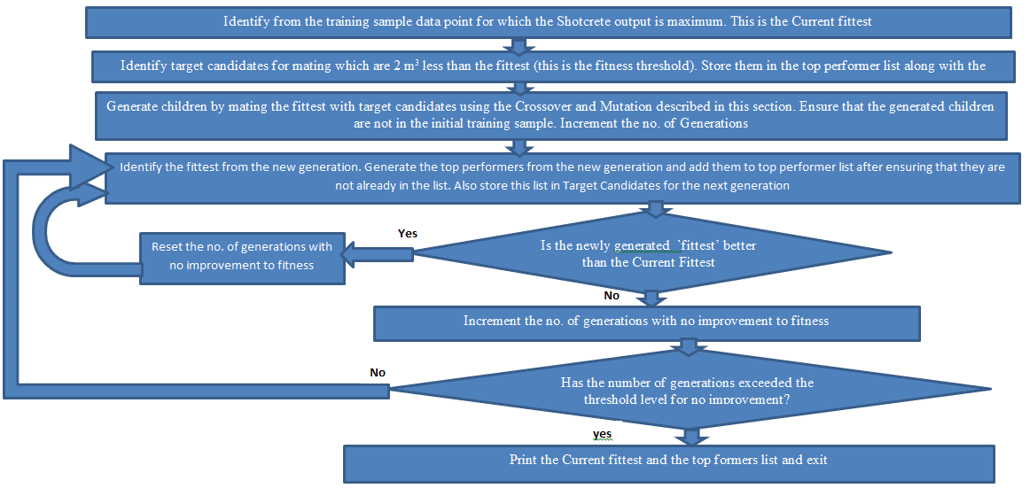
5. The Fittest and the Best Performers list
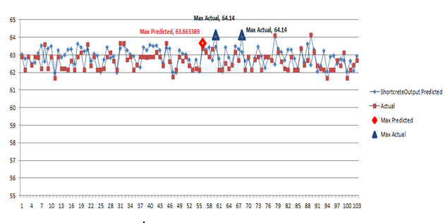
The algorithm was run starting from the training set. The fitness was found to improve for 2 generations followed by 10 generations (the threshold level) of no improvement The best performers list and the fittest candidate were generated using the algorithm above.
The following chart shows the plot of the predicted and the actual values of the Best Performers along with predicted and actual fittest candidates. As can be seen the predicted value very closely follows the actual behaviour and is quite reliable in identifying the attributes required for maximising Shotcrete output.
6. Conclusion
The objective of this paper is to demonstrate the process of developing a Deep Learning Model to predict and optimise parameters that would lead to maximising a process out. Shotcrete Process was taken as an example but the methodology is same for any other model construction. The following were the key learnings:
- Choice of the training set is also very important for building a close fit model. All possible variations need to be covered as described in 2 in order to discern the actual behaviour. This requires careful experimentation to gather the right data.
- Building neural networks requires some experimentation to emulate closely a nonlinear behaviour. There is always a trade-off between reaching global minima and minimising the error and over-fitting real time behaviour. One should train and test multiple hidden layers before arriving at the appropriate architecture.
- The number of epochs needed for training has to be a high value: 50,000,000 in this instance.
- Training to get to global minima requires adjusting learning rate and momentum. Effective training was achieved by setting learning rate and momentum to 0.1. Otherwise the “error on epoch” was found to increase after hitting a minimum value or oscillate about a value