
An Introduction to Bayesian Reasoning
You might be using Bayesian techniques in your data science without knowing it! And if you’re not, then it could enhance the power of your analysis. This blog post, part 1 of 2, will demonstrate how Bayesians employ probability distributions to add information when fitting models, and reason about uncertainty of the model’s fit.
Grab a coin. How fair is the coin? What is the probability p that it will land ‘heads’ when flipped? You flip the coin 5 times and see 2 heads. You know how to fit a model to this data. The number of heads follows a binomial distribution, and because 40% were heads, the most likely value of p is 0.4, right?
That’s almost certainly not the value of p, of course. You don’t really believe that you hold a biased coin, do you?
There are two ways to get to that answer, and you might be using one or both as a data scientist without being aware of it. This post will explore the frequentist and Bayesian way of looking at this simple question, and a more real-world one. We’ll see how the Bayesian perspective can yield more useful answers to data science questions because it lets us add prior information to a model, and understand uncertainty about the model’s parameters.
Maximum Likelihood Estimation and the Frequentists
p=0.4 actually is the best answer in a certain sense. Under the binomial model, it’s the p that makes the observed data most likely. It’s more likely to see 40% heads with a coin that lands heads 40% of the time than 50% or 10%. Knowing nothing else, the best guess is that 40% of future flips will land heads.
This approach seeks the value of the parameters (here: just p, the probability of heads, but more generically denoted θ) that makes the data most likely (here, the 2 out of 5 heads, but more generically denoted X). This is the maximum likelihood estimate (MLE) and is a so-called frequentist view of fitting a model. In the language of probability, that’s p(X|θ), and the goal is to find θ that maximizes it. This is attractive because here, p(X|θ) follows a simple binomial distribution, specifically Binomial(5,p).
That answer is unsatisfying, because it just seems unlikely that a normal-looking, government-minted coin is actually so biased. To do better, we need to capture that intuition.
Mean A Posteriori and the Bayesians
There’s another way to look at this: maximize p(θ|X). Given the data, why not find the maximum value of the parameter’s distribution? It sounds like the same idea, and sometimes leads to the same answer, but flips the problem around entirely.
But, what is p(θ|X)? It does not describe the probability of data, but the probability of a parameter. It doesn’t follow a binomial distribution. It turns out that it follows a beta distribution, and after seeing 2 heads and 3 tails, it’s common to analyze this distribution as Beta(3,4):
import numpy as np
 import scipy.stats as stats
 from matplotlib import pyplot as plt
x = np.linspace(0, 1, 128)
plt.plot(x, stats.beta.pdf(x, a=3, b=4))
plt.show()
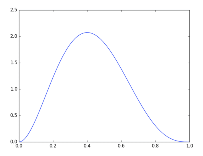
The most likely value occurs at the distribution’s “peak”, or mode, and this value is called the maximum a posteriori estimate (MAP). Fortunately the mode is easy to compute from its parameters. Plug in to the formula and find that it’s (3-1) / (3+4-2) = 0.4.
That obvious answer is sure sounding like the right one, but it still doesn’t feel right. One bonus of this approach is that it yields a whole distribution for the parameter, not a single point estimate. The wide dispersion of this distribution indicates a lot of uncertainty about the value of the parameter, when it doesn’t seem that uncertain.
Bayes’ Rule and Priors
There’s more to p(θ|X). Bayes’ Rule unpacks it: p(θ|X) = p(X|θ) p(θ) / p(X)
p(X) can be ignored for purposes of maximizing with respect to θ as it doesn’t depend on θ. It’s sufficient to maximize p(X|θ)p(θ). That’s merely what the MLE estimate maximizes, p(X|θ), times p(θ). The new term p(θ) is the probability of the parameter, irrespective of the data. That’s a problem and an opportunity. It can’t be deduced from the data. It’s a place to inject external knowledge of what the distribution of the parameter should be: its “prior” distribution, before observing data.
If we know nothing about θ, then all values of θ are equally likely, before. p(θ) is then a flat, uniform distribution. p(θ) becomes a constant, and maximizing p(θ|X) is the same as maximizing p(X|θ). That’s why the MLE and MAP estimates were the same; the MAP estimate implicitly assumed a flat prior, or, no prior knowledge about the parameters. That assumption is easy to overlook, and here it doesn’t sound right.
You do know something about coins in your pocket. You presumably believe they’re very likely to be very close to fair and unbiased.
It turns out that it’s convenient in this case to use a beta distribution again to represent that knowledge (technically: it’s an easy choice because it’s the conjugate prior for the binomial distribution). Recall the last 50 coins you’ve flipped in your life; let’s say that 27 were heads. That information could be encoded as a Beta(28,24) distribution.
With that choice, in this case, p(θ|X) will follow a Beta(30,27) distribution, and its mode is a satisfying 29/55 ≈ 0.527.
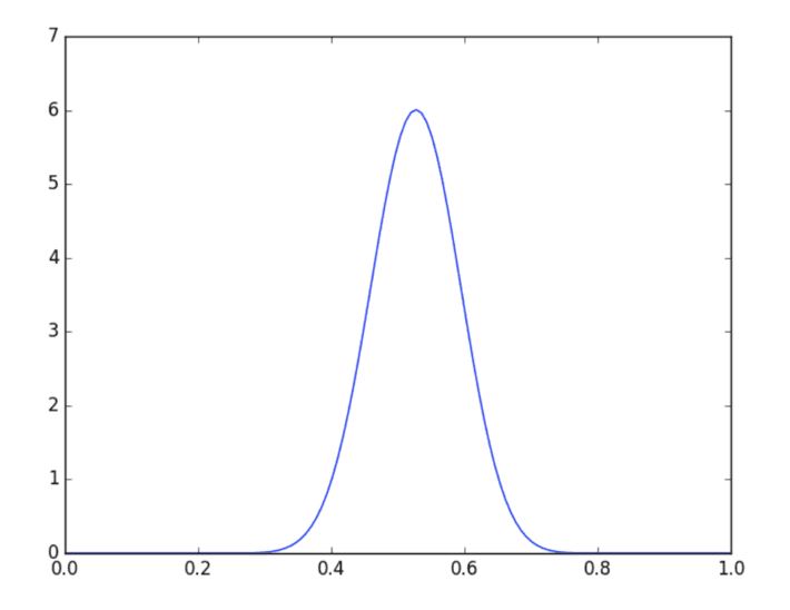
Values near 0.5 are much more likely under this analysis. The result matches expectations better because we injected our expectations! If the coin really was unfair, it would take much more evidence to overcome prior experience and make values of p far from 0.5 likely.
You may have noticed the beta distribution parameters map to the number of head and tails. Indeed the distribution of p after seeing h heads and t tails is Beta(h+1,t+1). This makes it easy to compute p(θ|X), which is called the posterior distribution, without any complex math. The new distribution is just a beta distribution with the number of heads and tails added to its parameters. This is the benefit of choosing a prior that is conjugate to the likelihood distribution of p(X|θ), because the posterior and prior are then of the same type, with related parameters.
Priors and Regularization
The Bayesian approach has some advantages over the MLE / frequentist approach:
- Can specify a prior distribution over parameters
- Yields a probability distribution over parameter, not just a point estimate
You may already be using these features without knowing it — in particular, priors.
If you’ve run a linear regression, you’re probably familiar with regularization. The common form of regularization, L2 regularization, penalizes large coefficients in the model by adding the square of the coefficients to the loss function being minimized. Why squared coefficients?
It turns out that this directly corresponds to assuming a prior distribution on the coefficients, a normal distribution with mean 0, and variance that corresponds to the strength of the L2 regularization. You’ve been asserting, with L2 regularization, that coefficients are most likely 0, and might be a little positive or negative, but probably aren’t very positive or very negative.
Here’s a simple regression on scikit-learn’s built-in “diabetes” data set:
from sklearn.datasets import load_diabetes
 import statsmodels.api as sm
 X, y = load_diabetes(True)
 sm.OLS(y, sm.add_constant(X)).fit().summary()
 ...
 ==============================================================================
 coef std err t P>|t| [95.0% Conf. Int.]
 ------------------------------------------------------------------------------
 const 152.1335 2.576 59.061 0.000 147.071 157.196
 x1 -10.0122 59.749 -0.168 0.867 -127.448 107.424
 x2 -239.8191 61.222 -3.917 0.000 -360.151 -119.488
 x3 519.8398 66.534 7.813 0.000 389.069 650.610
 x4 324.3904 65.422 4.958 0.000 195.805 452.976
 x5 -792.1842 416.684 -1.901 0.058 -1611.169 26.801
 x6 476.7458 339.035 1.406 0.160 -189.621 1143.113
 x7 101.0446 212.533 0.475 0.635 -316.685 518.774
 x8 177.0642 161.476 1.097 0.273 -140.313 494.442
 x9 751.2793 171.902 4.370 0.000 413.409 1089.150
 x10 67.6254 65.984 1.025 0.306 -62.065 197.316
 ==============================================================================
 ...
… and the same one with a little (alpha=0.01) L2 regularization (L1_wt=0):
sm.OLS(y, sm.add_constant(X)).fit_regularized(L1_wt=0, alpha=0.01).summary()
 ...
 ==============================================================================
 coef std err t P>|t| [95.0% Conf. Int.]
 ------------------------------------------------------------------------------
 const 150.6272 3.115 48.349 0.000 144.504 156.751
 x1 29.5706 72.266 0.409 0.683 -112.466 171.607
 x2 -11.9755 74.047 -0.162 0.872 -157.514 133.563
 x3 138.3663 80.471 1.719 0.086 -19.798 296.531
 x4 98.1438 79.127 1.240 0.216 -57.378 253.666
 x5 25.7808 503.971 0.051 0.959 -964.767 1016.328
 x6 13.1235 410.056 0.032 0.974 -792.835 819.082
 x7 -82.0492 257.054 -0.319 0.750 -587.285 423.187
 x8 77.7464 195.302 0.398 0.691 -306.116 461.609
 x9 124.9928 207.912 0.601 0.548 -283.655 533.641
 x10 72.9723 79.807 0.914 0.361 -83.886 229.831
 ==============================================================================
 ...
The coefficients are constrained by the prior and end up smaller in the second example. Although the model is not fit here with Bayesian techniques, it has a Bayesian interpretation. The output here does not quite give a distribution over the coefficient (though other packages can), but does give something related: a 95% confidence interval around the coefficient, in addition to its point estimate.
Conclusion
By now you may have a taste for Bayesian techniques and what they can do for you, from a few simple examples. Things get more interesting, however, when we see what priors and posteriors can do for a real-world use case. For part 2, please click here.