
Sometimes, you see a diagram and it gives you an ‘aha ha’ moment
Here is one representing forward propagation and back propagation in a neural network
I saw it on Frederick kratzert’s blog
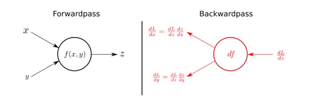
A brief explanation is:
Using the input variables x and y, The forwardpass (left half of the figure) calculates output z as a function of x and y i.e. f(x,y)
The right side of the figures shows the backwardpass.
Receiving dL/dz (the derivative of the total loss with respect to the output z) , we can calculate the individual gradients of x and y on the loss function by applying the chain rule, as shown in the figure.
A more detailed explanation below from me
This post is a part of my forthcoming book on Mathematical foundations of Data Science. Please follow me on Linkedin – Ajit Jaokar if you wish to stay updated about the book
The goal of the neural network is to minimise the loss function for the whole network of neurons. Hence, the problem of solving equations represented by the neural network also becomes a problem of minimising the loss function for the entire network. A combination of Gradient descent and backpropagation algorithms are used to train a neural network i.e. to minimise the total loss function
The overall steps are
- In the forward propagate stage, the data flows through the network to get the outputs
- The loss function is used to calculate the total error
- Then, we use backpropagation algorithm to calculate the gradient of the loss function with respect to each weight and bias
- Finally, we use Gradient descent to update the weights and biases at each layer
- We repeat above steps to minimize the total error of the neural network.
Hence, in a nutshell, we are essentially propagating the total error backward through the connections in the network layer by layer, calculating the contribution (gradient) of each weight and bias to the total error in every layer, and then using the gradient descent algorithm to optimize the weights and biases, and eventually minimizing the total error of the neural network.
Explaining the forward pass and the backward pass
In a neural network, the forward pass is a set of operations which transform network input into the output space. During the inference stage neural network relies solely on the forward pass. For the backward pass, in order to start calculating error gradients, first, we have to calculate the error (i.e. the overall loss). We can view the whole neural network as a composite function (a function comprising of other functions). Using the Chain Rule, we can find the derivative of a composite function. This gives us the individual gradients. In other words, we can use the Chain rule to apportion the total error to the various layers of the neural network. This represents the gradient that will be minimised using Gradient Descent.
A recap of the Chain Rule and Partial Derivatives
We can thus see the process of training a neural network as a combination of Back propagation and Gradient descent. These two algorithms can be explained by understanding the Chain Rule and Partial Derivatives.
Gradient Descent and Partial Derivatives
As we have seen before, Gradient descent is an iterative optimization algorithm which is used to find the local minima or global minima of a function. The algorithm works using the following steps
- We start from a point on the graph of a function
- We find the direction from that point, in which the function decreases fastest
- We travel (down along the path) indicated by this direction in a small step to arrive at a new point
The slope of a line at a specific point is represented by its derivative. However, since we are concerned with two or more variables (weights and biases), we need to consider the partial derivatives. Hence, a gradient is a vector that stores the partial derivatives of multivariable functions. It helps us calculate the slope at a specific point on a curve for functions with multiple independent variables. We need to consider partial derivatives because for complex(multivariable) functions, we need to determine the impact of each individual variable on the overall derivative. Consider a function of two variables x and z. If we change x, but hold all other variables constant, we get one partial derivative. If we change z, but hold x constant, we get another partial derivative. The combination represents the full derivative of the multivariable function.
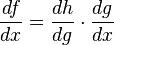
The Chain Rule
The chain rule is a formula for calculating the derivatives of composite functions. Composite functions are functions composed of functions inside other function(s). Given a composite function f(x) = h(g(x)), the derivative of f(x) is given by the chain rule as
You can also extend this idea to more than two functions. For example, for a function f(x) comprising of three functions A, B and C – we have
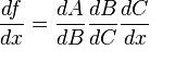
for a composite function f(x) = A(B(C(x)))
All the above, the elegantly summarised in this diagram
This post is a part of my forthcoming book on Mathematical foundations of Data Science. Please follow me on Linkedin – Ajit Jaokar if you wish to stay updated about the book