
For many, mathematical modeling is exclusively about algebraic models, based on one form or another of regression or on differential equation modeling in the case of dynamical systems.
However, this is too restrictive a point of view. For example, a clustering algorithm can be regarded as a modeling mechanism applicable to data where linear regression simply isn’t applicable. Hierarchical clustering can also be regarded as a modeling mechanism, where the output is a dendrogram and contains information about the behavior of clusters at different levels of resolution. Kohonen self-organizing maps can similarly be regarded in this way.
Topological data analysis is also an non-algebraic approach to modeling. In fact, one way to think about topological data analysis is as a new modeling methodology for point cloud data sets. As such, it is a very natural extension of what we usually think of as mathematical modeling.
The goal of this post is to discuss what we mean by mathematical modeling, and see how topological modeling fits with other modeling methodologies. In order to do this, let’s first observe that there are at least three important goals of a modeling system.
Compression: Any method of modeling should produce a very compressed representation of the data set, which is small enough for a user to understand. For example, linear regression takes a set of data points and represents it by two numbers, the slope and the y-intercept. The point is that most data sets contain too much information, and we need to strip away detail in order to obtain insight about the set.
Functionality: It should also allow users some actions based on the structure of the model. For example, linear regression permits the user to produce predictions of one or more outcome variables based on the values of independent variables
Explanations: The model should have the ability to explain its structure. For example, a clustering based model should have explanations about what distinguishes one cluster from another. Let’s discuss how these ideas work out for some different modeling methodologies.
Regression models
We mean here any method that approximates a data set by algebraic equations. It builds on the idea of analytic geometry, introduced by Descartes, in which compression of geometric objects is performed by recognizing that many geometric objects can be represented as solutions sets of equations. Approximating data sets by such geometric objects is then what constitutes the regression procedure. The output of such a model is an equation or a system of equations. The fact that there is compression is clear, since a geometric object consisting of infinitely many points can be represented by finitely many coefficients in an equation. It clearly provides functionality, in the form of predictive capability. Finally, it supplies explanatory information, for example by studying the coefficients of the variables to understand the dependence of an outcome variable on an individual independent variable.
While this case demonstrates that algebraic models can accommodate the goals of modeling system it is also important to note that algebraic models are often somewhat difficult to use for many kinds of data.
For example, consider the object below.

To represent this object algebraically requires equations of very high degree. What this means is that the degree of compression achieved is considerably less, since there will now be too many different coefficients which can be varied in the compression. This illustrates the point that, to be very informative, algebraic models need to be of relatively low degree, for example linear or quadratic. To be sure, one can do regression using families of functions other than polynomials, but that requires a choice of such a family. However, it is rarely clear which family of functions would be appropriate.
Cluster analysis
Cluster analysis is not often thought of as modeling, but in my view it should be. The output of a cluster analysis is a partition of the data into disjoint groups. In this case, the compression is achieved by providing the collection of clusters, which is typically small. This kind of compression often allows one to obtain understanding of phenomena that naturally fit in this paradigm, rather than the algebraic one.
For example, the division of diabetics into type 1 and type 2 cohorts, or division of voters into liberal, conservative, or independent are very useful conceptually, and this kind of behavior is very common in a large number of data sets. One can attach functionality to such a model by constructing a classifier that operates on a new data point and gives its best guess about which cluster the point belongs. In many cases, explanations can often be achieved. For example, if a data set consists of vectors with several entries or features, one can determine which of the variables best distinguish a given cluster from another one, or the given cluster from the entire data set, based on various statistical characterizations about the degree to which a variable distinguishes the clusters.
Hierarchical clustering
Hierarchical clustering is a particularly interesting methodology, since its output is a dendrogram, which is a subtler object than an algebraic equation or a partition. This modeling method was created to address the fact that many clustering algorithms require a choice of threshold, and it is often difficult to determine the right choice (if there is one) of the threshold. In this case, there is again compression, since one typically studies the high levels of the dendrogram, which produces a small number of clusters. In this case, there is also functionality in the model, since it can create clusters at every level, as well as determine the clusters at a higher level that contain a given cluster at a lower level. For example, in a clustering describing a taxonomy of animals, one can have a picture that looks as follows:
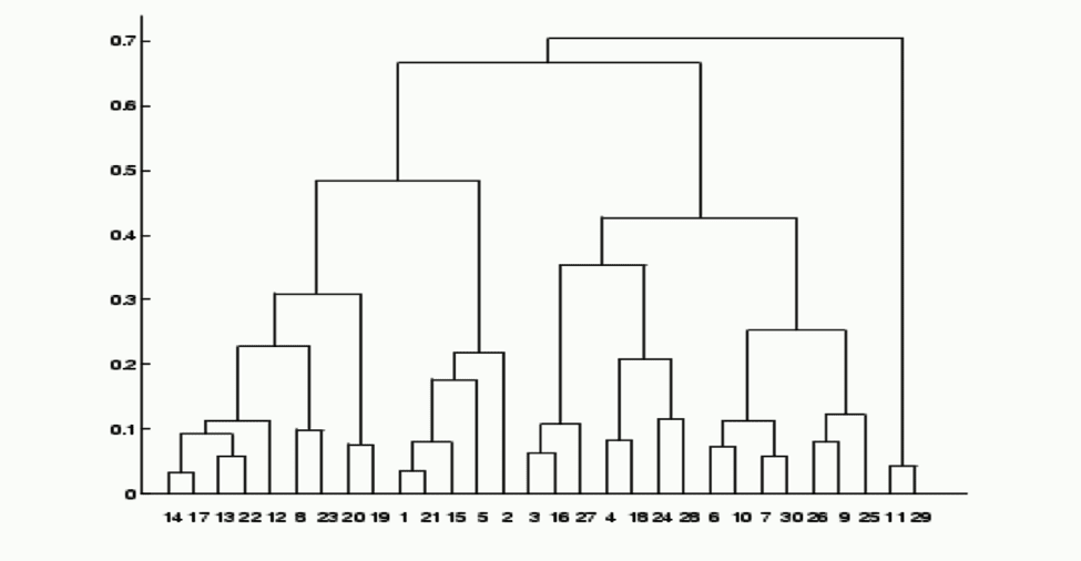
This is clearly an improvement over clustering at one or the other of the levels, since it encodes the fact that, say, Carnivora, Cetacea, and Chiroptera all belong to the higher level group of mammals.
Topological modeling
This is the methodology developed by Ayasdi. It produces as an output a topological network instead of algebraic equations, partitions, or dendrograms. It provides a great deal of compression of the data, since each node of the network corresponds to a (possibly large) group of data points, and the edges correspond to the intersections of these subgroups. It also provides a great deal of functionality, including the following possibilities:
- Layout of the network on the screen for visualization and unsupervised analysis.
- The ability to select subgroups of the data set by selecting groups of nodes, using standard gestural techniques such as lassoing.
- Given a group or pair of groups, determining the “explanatory variables” for the group vs. the rest of the data set or vs. the second group.
- The ability to color the network by a quantity of interest, by coloring each node by the average value of the quantity on the points in the collection corresponding to the node.
- Given a group defined externally, the ability to color each node by the fraction of the members of the corresponding group which belong to the externally defined group.
- Creation of new features associated to the network structure. This can include analogues of “bump functions” based on groups, centrality measures in the graph distance, and others.
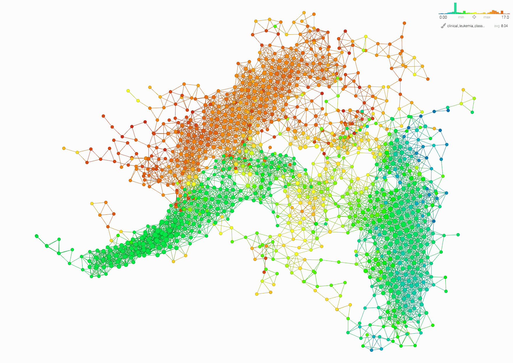
Within this topological model, four distinct leukemia subgroups are visible (they are colored orange, green, yellow and greenish-blue. The various leukemia types are numbered and the topological model subgroups are colored by the average value of the leukemia types in each group. From left to right, the orange group primarily contains ALL and B-ALL types, the green group is almost pure CLL, the yellow is AML and T-ALL derivatives and the bluegreen group is MDS and CML derivatives.
These primitive capabilities can be used in conjunction with each other to create methods to:
- improve predictive models
- deliver principled dimensionality reduction based on the data set’s network model structure
- develop hot spot analysis for understanding the distribution of a quantity of interest or a predefined group within the data set.
As for the explanations, the ability to color the network by a quantity of interest (#3 above) permits the explanation of various groups and the distinction of the groups in terms of the most distinguishing variables.
The main point to be made here is that mathematical modeling is not restricted to a small number of mathematical techniques, but should instead be viewed as the science (and art) of representing data by informative mathematical models of various kinds. Virtually all disciplines in mathematics contain kinds of objects that can serve as useful models in various domains. The key point about any methodology is the amount of insight it yields, and the extent to which it enables and speeds up the work of data scientists trying to extract knowledge from the data.