
Introduction
Data Science and Machine Learning are furtive, they go un-noticed but are present in all ways possible and everywhere. They contribute significantly in all the fields they are applied and leave us with evidence which we can rely on and take data-driven directions. Today, a very interesting area we are going to see an example of Data Science and Machine Learning is ‘Crimes’. We are going to focus on types of crimes taken place across 50 states in the USA and cluster them. We cluster them for the following reasons:
- To understand state-wise crime demographics
- To make laws applicable in states depending upon the type of crime taking place most often
- Getting police and forces ready by the type of crime done in respective states
- Predicting the crimes that may happen and thus taking measures in advance
The above are the few applications which can be considered but they are not exhaustive, depending upon the data reports produced by the algorithms there can be more such applications which can be deployed. Our concern today is to understand how we can deploy Hierarchical clustering in two ways i.e. DIANA and AGNES for the USA Arrests data.
Theory
Hierarchical Clustering
A clustering algorithm that groups similar objects in the form of clusters. The scope for a detailed understanding of Hierarchical clustering in this blog is not feasible as it is a vast topic. To get a detailed understanding of Hierarchical clusters follow this link.
By hitting the above link you will understand in and out of hierarchical clusters concerning their formation, the role of density and distances in hierarchical clustering with visuals diagrams. What we will focus today is on DIANA and AGNES hierarchical clustering.
DIANA Hierarchical Clustering
DIANA is also known as DIvisie ANAlysis clustering algorithm. It is the top-down approach form of hierarchical clustering where all data points are initially assigned a single cluster. Further, the clusters are split into two least similar clusters. This is done recursively until clusters groups are formed which are distinct to each other.
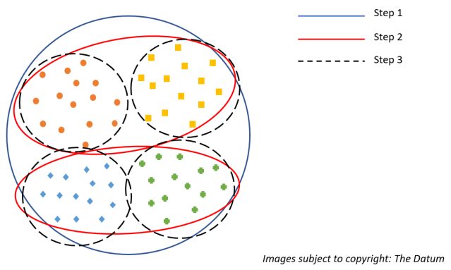
Notional representation of DIANA
To better understand consider the above figure, In step 1 that is the blue outline circle can be thought of as all the points are assigned a single cluster. Moving forward it is divided into 2 red-colored clusters based on the distances/density of points. Now, we have two red-colored clusters in step 2. Lastly, in step 3 the two red clusters are further divided into 2 black dotted each, again based on density and distances to give us final four clusters. Since the points in the respective 4 clusters are very similar to each other and very different when compared to the other cluster groups they are not further divided. Thus, this is how we get DIANA clusters or top-down approached Hierarchical clusters.
AGNES Hierarchical Clustering
AGglomerative NESting hierarchical clustering algorithm is exactly opposite of the DIANA we just saw above. It is an inside-out or bottoms-up approach. Here every data point is assigned as a cluster initially if there are n data points n clusters will be formed initially. In the next iteration, similar clusters are merged (again based on the density and distances), this continuous until similar points are clustered together and are distinct for other clusters.
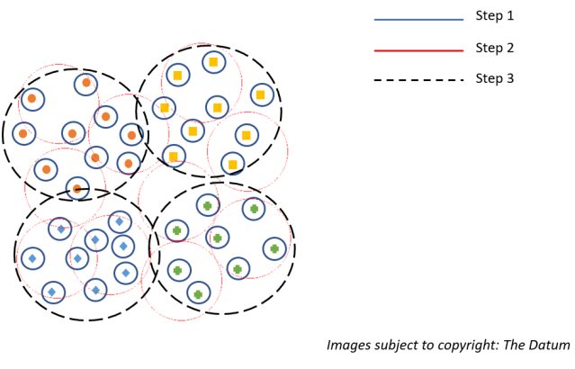
Notional representation of AGNES
As we can infer from the above representation for AGNES in step one all the data points are assigned as clusters. In step two again depending upon the density and distances the points are clubbed into a cluster. Lastly, in step 3 all the similar points depending upon density and distances are clustered together which are distinct to other clusters thus forming our final clusters.
With so much theory and the working idea of DIANA and AGNES Hierarchical Clustering, we can now move on to build our model in R.
The Model
Data
The data we are using today for modeling is an inbuilt R data in the MASS library. The data is named as ‘USArrests’, it has 50 observations (for 50 US States) with 4 variables or data fields. It has arrests per 100,000 residents (the Year 1973) for 4 different data fields which are as follows:
- $Murder – numeric – Murder arrests per 100,000
- $Assault – integer – Assault arrests per 100,000
- $UrbanPop – integer – Percent Urban Population
- $Rape – numeric – Rape arrests per 100,000
Below shows the listing for loading the library followed by loading the USAssaults data set. Later images show the summary and structure of data set generated in R.
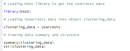
Loading Data in R
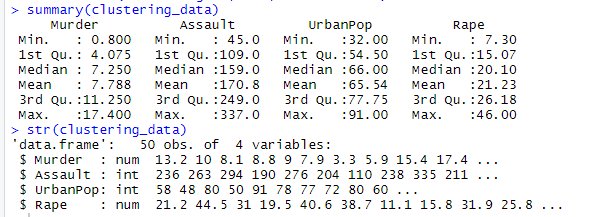
Summary and Structure of USArrests
Hopkins Statistic
Okay, we know we are clustering but, are we sure the data we are performing clustering can be clustered? Will the clusters that will be formed will be valid? To get answers to this question we will compute Hopkins Statistic. It is a measure to determine cluster tendency, the tendency takes a value between 0 and 1. And the cut off for our useful value is below 0.5, if the Hopkins statistic computed is below 0.5 then clusters are likely to be formed and valid clusters and if over 0.5 and closer to 1 the structures are not valid in the data set and are random.
The ‘factoextra’ library has the function get_cluster_tendency() {load the library factoextra} this functions returns the Hopkins Statistic for the data. Below is the listing to compute the clustering tendency followed by the Hopkins static obtained.
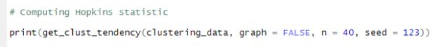
Listing for computing Hopkins Statistic
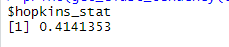
Hopkins Statistic obtained
Since we obtained Hopkins statistic of less then 0.5 which is equal to 0.4141 we can say that the structures in the data set are not random and are real structures out of which clusters can be formed.
Determining ‘k’
The next big question to answer is what should be the optimal k value i.e. the number of clusters which are to be formed. There will be scenarios where you will be directly given a ‘k’ value depending upon the application. And there are as many as 30+ ways to determine this k-value. The most efficient and excellent way which is making use of NbClust() function of R library. It determines the optimal number of clusters by complex computations by varying all combinations of several clusters, distance measures, and clustering methods all at once. Once all the computations are done the output of k-value is given by majority rule. We can hence use the computed k-value. Below is the listing to compute k value using NbClust(). You may have to install followed by loading of NbClust() if not already in use.
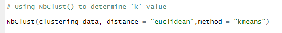
Deploying NbClust()
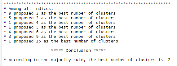
Snippet of the summary generated by NbClust()
As we can see above, NbClust suggests the optimal number of clusters should we form must be 2. Thus, we will go ahead with this value as k.
Modeling DIANA
Now, we can proceed to model DIANA. For this, we will first load the library Cluster which has the function for both DIANA and AGNES. Below is the listing for computing DIANA and plotting dendogram of DIANA using pltree function.
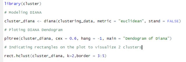
Listing for computing and DIANA and plotting DIANA dendogram
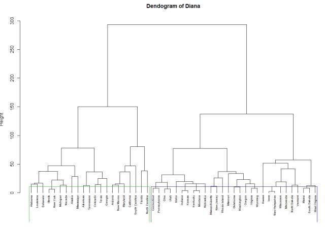
Dendogram of DIANA, with rectangles indicating 2 clusters
For DIANA we have a metric called as divisive co-efficient which can be extracted as an attribute from the DIANA model formed as $dc. This is the measure which takes a value between 0 and 1 and closer to 1 the better.
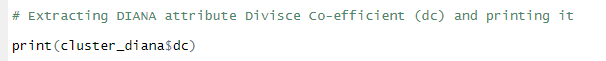
Listing for extracting DIANA attribute $dc
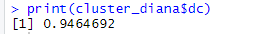
Obtained Divisive co-efficient $dc
As we can see above the $dc value obtained is very close to 1 thus we can say the clusters are accurately formed and are valid. Now to see the names of the actual clusters formed and their relationships we use function cutree() that groups the clusters which we can use to print the clusters and see the cluster relationships.
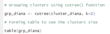
Using cutree() function to group clusters formed in DIANA
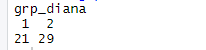
Cluster Sizes of DIANA
As we can see from above Cluster 1 has 21 states and cluster 2 has 29 states clustered both making up to 50 states. Further, we can print the clusters and see the relationships between them and understand why the clusters were formed the way they were. Below is the listing for creating a function to print the clusters, followed by printing the DIANA clusters.
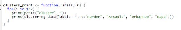
Listing for creating a function to print the clusters
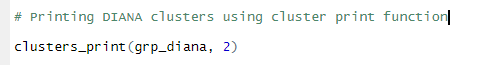
Printing clusters using cluster print function
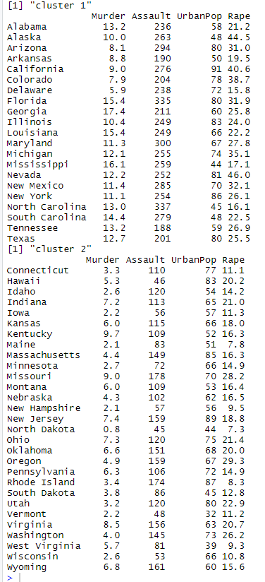
Print of DIANA Clusters
In general comparison of the above two clusters, we can infer that the states are generally divided into two groups. The first group of states in cluster 1 are the states that have high murder, assault and rape cases per 100,000 compared to the states of cluster 2. Below is the mean comparison of Murder, Assault and Rape cases of both the clusters.
| Murder | Assault | Rape | |
| Cluster 1 | 11.8 | 255 | 28.1 |
| Cluster 2 | 4.7 | 109.7 | 16.2 |
Thus, from so much inference we can understand that cluster 1 states have more average arrests per 100,000 compared to cluster 2 states. Cluster 2 states are safer then cluster 1 states.
Lastly, we will visualize the clusters, we can visualize the cluster results using the function fviz_cluster() from the factoextra library. The plot is in two dimensions and is based on the first two Principal Components that explains the majority variance. Following is the listing for visualization
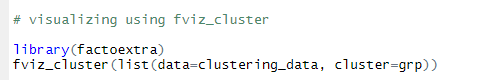
Listing for visualizing DIANA clusters
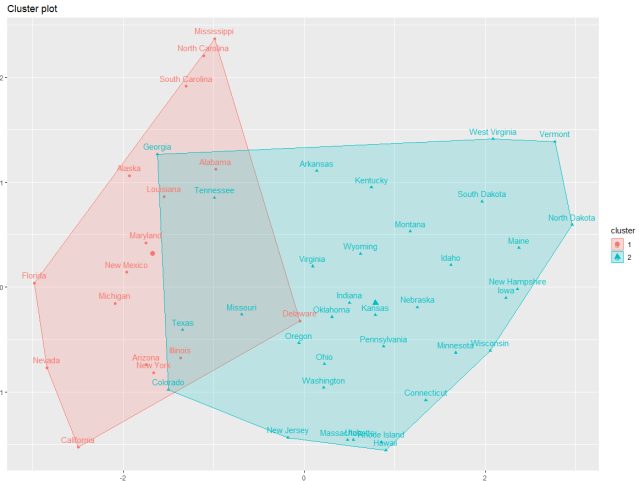
DIANA clusters – Visualization
Modelling AGNES
So far whatever we have done for DIANA we will be executing the same for the AGNES clusters as well. Below is the entire listing for modeling, evaluating and visualizing AGNES clusters. Please refer the comments in the listings to get the idea about the listings.
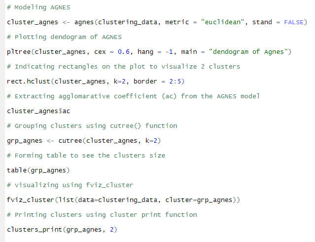
Listing for modelling, evaluating and visualizing AGNES
As we saw dc co-efficient in DIANA we have ac (agglomerative coefficient) for AGNES. Again, takes a value between 0 and 1. The closer to 1 the better and here we have 0.90 which is a good ac value indicating the clusters formed can be relied upon.
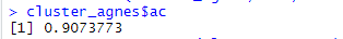
ac co-efficient of AGNES
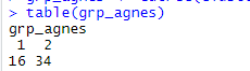
Cluster table of AGNES
Below is the print of clusters formed by AGNES
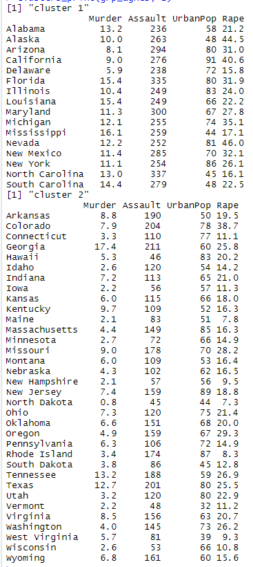
AGNES Clusters print
AGNES clusters summary:
| Murder | Assault | Rape | |
| Cluster 1 | 11.8 | 266.3 | 28.3 |
| Cluster 2 | 5.8 | 122.8 | 17.8 |
As we can see from the above summary table of clusters, AGNES has formed clusters which are relevant to DIANA in the sense that Cluster 1 states have a higher number of murder, assaults, and rape per 100,000 compared to the states of cluster 2.
Below is the fviz_cluster() plot for AGNES
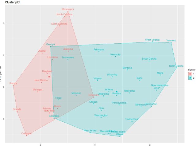
AGNES cluster plot
Takeaways
- Make use of Hopkins statistic to realize the relationship in the data is random or real to form clusters. It should be below 0.5
- No matter which approaches to take either DIANA or AGNES both will give you clusters with same meaning just the number of entries in the clusters might differ
- Both are easy to compute and visually you can view the dendogram to understand both of the clusters
- Make use of fviz_cluster function to visually compute clusters in the first two principal components where majority of information lies
Conclusion
Clustering is an unsupervised machine learning algorithm in which we compute analytics mostly without a pre-defined aim to understand the relationships between the data. Once we get the understanding and trends in the data we can accordingly take necessary actions and data-driven decisions. In this case, viewing the states in cluster 1 there can be more strict law enforcement in the cluster 1 states to reduce the number of murders, assaults or rape cases. Police and officials can be more equipped and trained for such situations as well.
EndNote
Datum was started with a vision to give the thoughts and working of Data Science and Machine Learning Algorithms. Continuing with this vision The Datum is growing and getting better and would like to thank all the supporters, followers and viewers from more than 65 countries worldwide. We at Datum appreciate this and hope we get continued support.
Multiple Datum’s form Data, mindless Data can do wonders. Mindful you and I together can do magic! A source where you can gain/contribute Data Science, Because together we can get better!
Your Data Scientifically,
The Datum
Read more here.