
I wrote this article for machine learning and analytic professionals in general. Actually, I describe a new visual, simple, intuitive method for supervised classification. It involves synthetic data and explainable AI. But at the same time, I describe in layman’s terms the Riemann Hypothesis (RH). Also, I offer a new perspective on the subject for those who attempt to solve the most famous unsolved mathematical problem of all times. I included the Python code to generate the videos, producing some of the most beautiful orbits.
Introduction
On YouTube, you can find many videos about RH, including mines. Most are produced by mathematicians. Typically, they don’t do a great job at explaining the topic to a large audience. Foremost, I am a machine learning scientist. So my perspective is different. While I try to come up with machine learning techniques that are math-free and model-free (this is also the case here), my datasets require good math knowledge to produce. Also, I spend a lot of time developing ML algorithms to gain insights on advanced math problems.
This article summarizes my most recent progress in this direction. Hopefully, it will entice the reader to further explore RH, its mathematical beauty, and potential applications to ML. It is a continuation in a series of articles: you can find some of the previous ones on Data Science Central, here and here.
The Riemann Hypothesis in a Nutshell
Possibly the simplest way to introduce RH, yet with enough math to fully grasp the problem and start your own original research, is to start with the Dirichlet eta function η(z) in the complex plane. Here z = σ + it is a complex number. But you don’t need to know anything about complex numbers: z is simply a vector (σ, t). The horizontal axis is the real one, and the vertical axis is the imaginary one. In other words, σ is the real part of z, and t the imaginary one. Also, t represents the time, when plotting an orbit of η(z) for a fixed value of σ.
The η function accepts complex arguments z and returns complex values η(z). The real and imaginary parts of η(z) are respectively:
\begin{align}
\eta_X(z) & = \sum_{k=1}^\infty (-1)^{k+1} \frac{\cos(t\log\sigma)}{k^\sigma}\\
\eta_Y(z)& =  \sum_{k=1}^\infty (-1)^{k+1} \frac{\sin(t\log\sigma)}{k^\sigma}\\
\end{align}
The reason to work with η(z) rather than its sister — the Riemann zeta function ζ(z) — is that the above series converges if σ > 0. To the contrary, the series for ζ(z), where -1 is replaced by +1, converges only for σ > 1. Yet all the interesting action takes place when 0.5 ≤ σ < 1. We also have
\eta(z) = (1-2^{1-z})\prod_{p}\frac{1}{1-p^{-z}} = (1-2^{1-z})\zeta(z),where the product is overall prime numbers. Again, the product converges only if σ > 1. Thus the η function is used to extend the definition of ζ to σ > 0. The two functions η and ζ have the same roots if 0 < σ < 1. The Riemann Hypothesis states that all these roots lie on the line σ = 0.5, called the critical line. The band 0 < σ < 1 (in the complex plane) is called the critical strip.
Visualizing the Orbits
Figure 1 visually explains RH. It is the last frame of a Python video, viewable on YouTube, here. The left black dot on the X-axis is the origin; the right one is (1, 0). There is a circular area around the origin that the blue orbit never hits or crosses. Same with the yellow orbit, though the corresponding area is larger and further to the right: the center of the empty zone is not the origin in this case. On the contrary, the red orbit has no such area; indeed the origin is an attraction point.
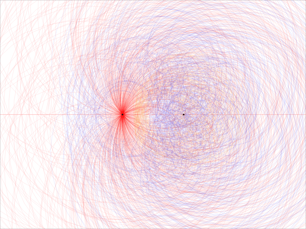
An empty zone inside an orbit is called a repulsion basin in dynamical systems. Let’s use the word “hole” instead. Since the origin is inside the hole of the blue orbit, η(z) has no root if σ = 0.75. The same is true for any value of σ strictly between 0.5 and 1. This is equivalent to RH! Note that the orbits in Figure 1 are displayed only for 0 < t < T, with T = 1,000. The more you increase T, the more the hole shrinks. In the end, when you display the entire orbit (when T is infinite), the hole shrinks to either a single point (the origin) or an empty step. Whether it is a single point or an empty set, nobody knows. RH states that the hole becomes a single point, not an empty set.
The implications are enormous. There is a one million dollar award to solve this problem, offered by the Clay Institute. Finally, any tiny modification to η(z) results in losing the hole entirely. There is very little leeway here. Other functions with the same behavior exist, but they are not common.
Visual Supervised Classification
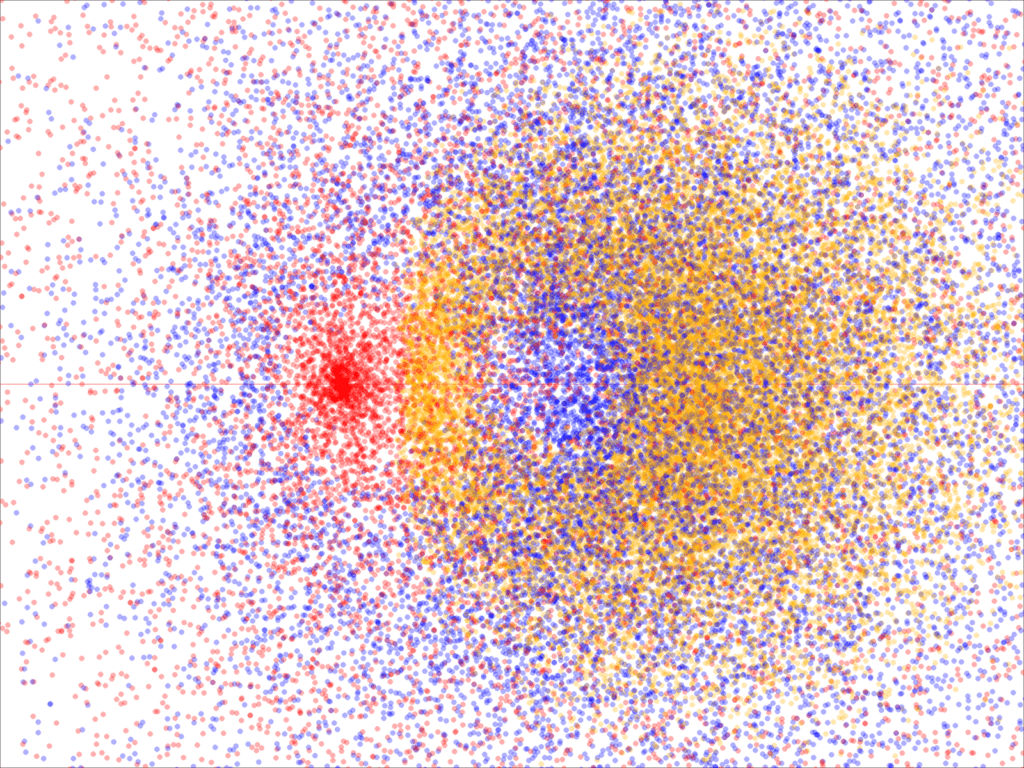
To produce the orbits, I used evenly spaced values of t. If you look at the video, the orbits move at varying velocities depending on t, resulting in uneven point densities. You can correct that, using uneven sampling. Either way, you end up with a set of points in two dimensions. Now you can perform supervised classification: assigning a color to an arbitrary location in the 2D space.
The dataset is a challenging one. This is due to massive cluster overlapping, bounded and unbounded clusters (the yellow one is bounded, the other ones are not), and holes in the blue and yellow clusters. You can use the dataset to benchmark different classification algorithms. For some locations, you can tell that the label is either red or yellow with some probabilities, but not blue. It is similar to saying you don’t know with certainty what disease the patient has, but you can rule out cancer. Bayesian classifiers seem particularly appropriate in this context.
Details about the Classifier
My classification algorithm requires first to map the dataset into an image bitmap. Then you apply convolution filters — an image processing technique — to perform the classification of the entire window (or at least, a large portion of it). You can do it in GPU. It generalizes to more than two dimensions, using tensors. The result is pictured in Figure 2. The full description, including Python code for classification and producing the videos, is available here and here. The Python code also produces the data sets. A video, showing the classification in progress, is available here.
The core of the methodology uses blending colors and transparency levels, to perform the classification. In the end, the classifier is a neural network in disguise: the pixels are the neurons, and the weights in the convolution filter are the parameters of the neural network. If you filter the entire image multiple times, each full iteration corresponds to a layer in a deep neural network. The whole procedure allows you to classify a new point very fast, but it uses a lot of memory.
About the Author
Vincent Granville is a machine learning scientist, author, and publisher. He was the co-founder of Data Science Central (acquired by TechTarget) and most recently, the founder of MLtechniques.com.