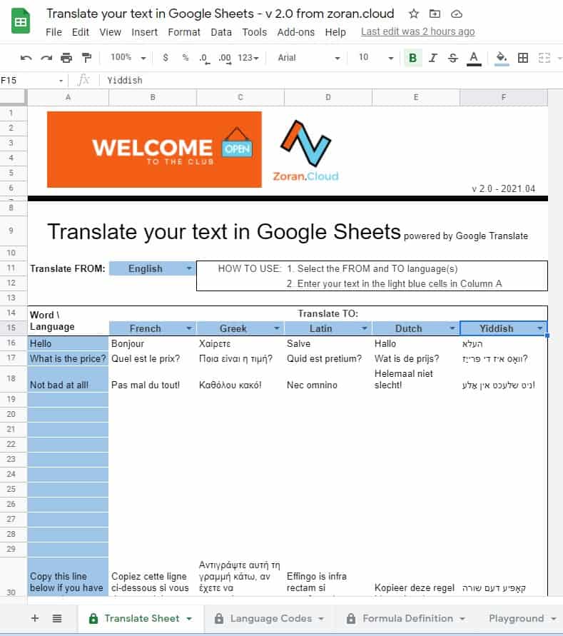
Google Translate is an amazing feat of engineering, which uses artificial intelligence to translate speech and text from a chosen language into another. In most cases, Google Translate’s own interface embedded in Google Search or on translate.google.com suffices to get some ad-hoc thing translated quickly.
Again, as in other Case Studies presented here, Google Sheets comes to the rescue!
Main formula:
=GOOGLETRANSLATE(B16, “en”, “fr”)
- Here, the ‘B16’ part concerns the reference to the cell containing the text you want to translate.
- After that, you add the source language — the language in which the original text is written — using the language’s abbreviation.
- After that, you declare the target language — the language to which the source text has to be translated — again using that language’s abbreviation.
How to make this even better?
1. Drop-down lists for the languages
Other than formatting the file to your liking, you can create some drop-down lists for the Source and Target languages.
This will help you being more productive as you do not need to search for the language codes every time you want to change them.
In my case, I used the Data Validation feature using as a criterion a List from a Range. First, I created a new sheet with all the Languages and their codes. Then, I used the column with the language names as my List for data validation.
Advantages of the drop-down list:
- It can be sorted (in my case, I used the alphabetical sort in the Language Codes Sheet).
- It is searchable.
- Can auto-update if your data changes – see the TIP below
For your drop-down list to auto-update when you are adding new data on the criterion Range, use a formula like: =’Language Codes’!$A$2:$A
Note that on the range defining the data that will be used for the drop-down list, I specify the beginning of the selection ($A$2: row 2 of column A) but I do not specify any row at the end of the selection (:$A).
I could have written the formula like this =’Language Codes’!$A$2:$A65 but then, every time I am adding new languages to the list I will need to update the Data Validation formula.
2. VLOOKUP function to pick the language code
I have now the Language selected from the drop-down list but in the formula I need to have the Language Code and not the language name. Therefore, I am using the VLOOKUP function that is searching the Language Name in the Language Code Sheet and returns the Language Code corresponding to the selection.
VLOOKUP($B$11,’Language Codes’!A:B,2,FALSE) – Source Language
So it looks for the value in cell B11 (the source language) in the Sheet “Language Codes” on column A. Once it finds the Language, it will return the information on the next column on that specific row. The Language Code. If the language is set to English, this function will return “en”.
VLOOKUP($B$15,‘Language Codes’!$A:$B,2,FALSE) – Target Language
It looks for the value in cell B15 (the target language) in the Sheet “Language Codes” on column A. Once it finds the Language, it will return the information on the next column on that specific row. The Language Code. If the language is set to French, this function will return “fr”.
So, starting from the formula definition on the yellow area, our complete formula will look like this now (check the color code on the formula definition to spot every part):
=GOOGLETRANSLATE(A16,VLOOKUP($B$11,‘Language Codes’!A:B,2,FALSE),VLOOKUP($C$15,‘Language Codes’!$A:$B,2,FALSE))
3. CLEAN ERRORS PROACTIVELY
Since we pre-populated the entire table with formulas, the rows where we do not have a text to be translated will bring an error message #VALUE! It is not an error per se but it will make our file look ugly. Therefore, we can use the =IFERROR function and instruct Google Sheets to discard all the errors and show instead of an empty cell.
Since the function definition is =IFERROR(value, [value_if_error]), we will have to
- replace the value part with out formula defined above
- replace the value_if_error part with “” – this is a way to writing an empty text … nothing between the quotation marks
Final formula:
=iferror(GOOGLETRANSLATE(A16,VLOOKUP($B$11,‘Language Codes’!A:B,2,FALSE),VLOOKUP($B$15,‘Language Codes’!$A:$B,2,FALSE)),“”)
Yes, we are done. We will not complicate the formula more than that.
Register for FREE on https://zoran.cloud to use the Google Sheet file. If you want to make any changes or have it on your own Google Drive account, make a copy, use it and abuse it :-).
Zoran

