
I’m unsure if it is a common misconception, but I know I used to believe that the only thing needed to present findings from statistical analysis was a P-value less than the chosen alpha; that if there was evidence to reject the null hypothesis it could be concluded that a meaningful discovery had been made. What I learned during the Mod 3 project is that statistical significance is not indicative of a substantive significance in what is being measured or compared. In order to determine the true impact of a test drug on treatment or a new webpage design on sales, etc., it is important to also calculate effect size.
Effect size is a quantitative measure of the strength of a test group and is a description of the size of the difference or relationship between two compared samples. Picture two normal bell curves, representing two samples one is comparing. Imagine the samples have the same mean, so the curves lay atop one another. Now imagine that the mean of the alternate sample, the group hypothesized to have some statistical difference than a control group, increases. The alternate bell curve begins to slide along the x-axis away from the control curve and the distance between the vertical lines in the middle of each curve (representing their means) begins to widen. That gap between their means is the effect size.
It is important to be able to present the effect because that will provide tangible value to statistical findings. An example is a restaurant owner wanting to know if she should renovate her New York City based location. The renovation will cost $100,000 and the owner needs to know if the cost will be covered by new business the renovation brings. A data scientist is contracted to see if renovated restaurants conduct more business than those left unrenovated. Data is collected and a t-test is run that finds a significant p-value, stating that yes, renovated restaurants do fair better. However, until the data scientist determines the effect size between the sample means, it would not be known if renovations return an additional $200 in annual revenue or an additional $200,000. The analysis would not offer the business owner the full picture about their investment.
A common way to calculate effect size is to find Cohen’s d term. d is calculated by taking the difference in means of two samples divided by the standard deviations of the samples. Cohen determined d values of 0.2, 0.5, and 0.8 to denote small, medium, and large effect sizes, respectively. When comparing samples from different groups – e.g. test scores from students at schools in California vs students from Michigan – the samples might have different variance so standard deviation is pooled for the denominator.
When two samples have an effect size of 0, the mean of the alternate group is at the 50th percentile of the control group and the bell curves would completely overlap. With an effect size of 0.8, the mean of the alternate group falls at the 79th percentile of the control group, so an average case of the alternate group would be higher than 79% of the control group.
Absolute effect size can be useful when the units of the means we are comparing are well known – something like distance or cost. When presenting information on data that is comparing means of something with less meaning to a general audience, we can best understand effect size by calculating a standardized measure of effect, which transform the effect to a digestible scale. This could be useful if you were comparing the magnitudes of earthquakes in various regions of the world and wanted to determine how significant a difference was in their measure on the Richter scale.
An additional metric that can be used when describing the outcome of statistical analysis when comparing two groups is Power. Power is a product of many things but what it tells us is how likely we are to reject the null Hypothesis when it is false, thereby giving Beta, the likelihood of committing a Type II error. Power considers effect size, the chosen alpha, and the sample size, and determines how often will we be able to find a statistically significant outcome that will provide enough evidence to reject a false null hypothesis (which is what any good statistician wants!). A generally acceptable level for power is 80% – if you cannot produce a power level of at least 80%, many statisticians would suggest you should not continue with the analysis.
Here is a quick refresher on the potential outcomes of a statistical test and how α and β play in:
|
Null Hypothesis is: |
|||
|
True |
False |
||
|
Judgement of Null (Statistical Result) |
Reject Ho (p<.05) |
Type I Error False Positive α |
Correct inference True positive (1 – β) |
|
Fail to reject (p>.05) |
Correct inference True negative (1- α) |
Type II Error False Negative β |
|
Where α is alpha (probability of Type I Error) and β is beta (probability of Type II Error)
A data scientist does not control the effect size, as that is dependent on the means of the two groups. However, a larger effect size will lead to a higher power of the significance test and reduce the probability of making a Type II Error (β). Because power = (1 – β), so if power goes from .8 to .9, that would be a reduction in β, the P(Type II Error) goes from .2 to .1.
Operating with a lower power can present a problem when conducting study replication because we would treat a replication as an independent occurrence and have to multiply powers to find a combined likelihood of finding real effect. E.g. if both the original and the replication studies both have a power of 80%, then we are only 64% likely to detect a real effect in both.
A helpful acronym to remember methods to increase the power of a test is APRONS. APRONS stands for:
- Relax alpha level
- Use a parametric statistic
- Increase the reliability of the measure
- Use one tailed test
- Increase the sample size(n)
- Increase the sensitivity of the design and or analysis
Below are some visual examples of how relaxing the alpha level and increasing the sample size increase power:
Given a sample of 20, an alpha level of 0.05, and a calculated effect size of 0.63 (a relatively medium effect size), you can see we are sure that the given sample size will help us avoid throwing a Type II error 80% of the time (power presents as the light blue shaded region):
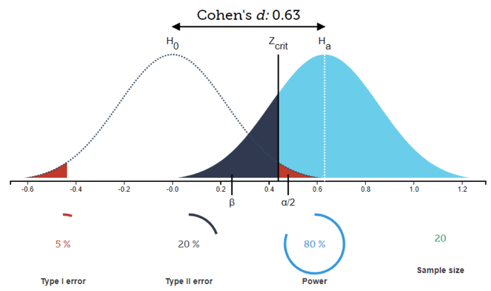
Fig. 1
If we increase the acceptable rate for a Type I error by increasing alpha to 0.1, we see that power increases to .88:
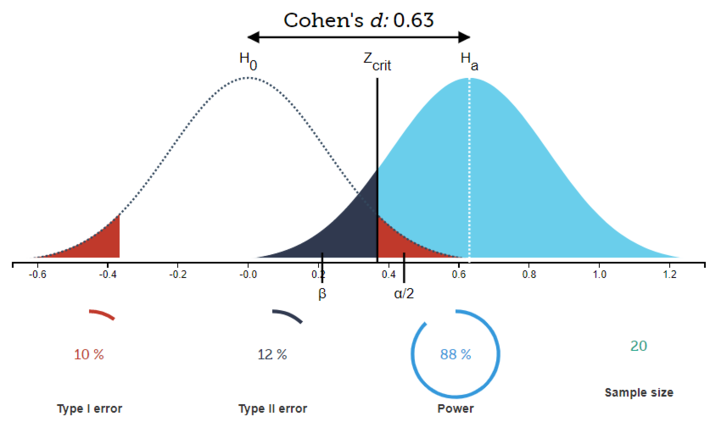
Fig. 2
By increasing alpha, we are pulling the Zcrit line to the left, thereby increasing the amount of the alternative distribution that lies to the right of the Zcrit threshold.
And finally, if we were to maintain our alpha level, we could also choose to increase sample size to 30, thereby increasing power from .8 to .93:
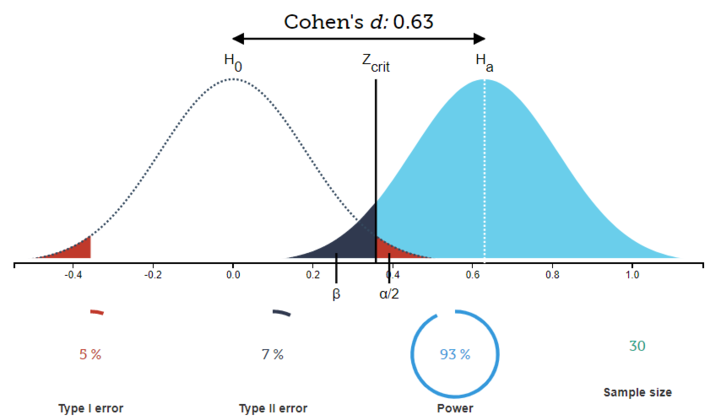
Fig. 3
By increasing sample size, one can effectively decrease the standard error between the two groups and reduce the amount of overlap between them, which will also cause the range and variability of the sample distributions to decrease.
While using Python, one can use the TTestIndPower method, found in statsmodels.stats.power package, to input three known metrics of alpha, effect size, desired power, and sample size in order to determine a fourth. The method completes Statistical Power calculations for t-test for two independent samples using pooled variance.
Hopefully this provides a better idea of why calculating effect size and knowing the power of a test is important for statistical analysis.
Sources:
Information on p-value: https://www.ncbi.nlm.nih.gov/pmc/articles/PMC3444174/