

I. Introduction
This project involved implementing machine learning methodologies to identify similarities in job skills contained in resumes. An organization presented the project to the New York City Data Science Academy to explore whether Academy students might be interested in working on it. The three authors of this post, all students at the Academy at the time, agreed to take the project on. In formulating the analysis described in this post, the authors collaborated with several representatives of the organization. While the organization has asked us to refrain from disclosing its name at this time, the authors wish to convey their gratitude to the organization for the opportunity to work on the project as part of our studies at the Academy.
The general idea underlying this project was to uncover semantic similarity and relations behind skills that appear on resumes. A semantic-based approach to evaluating job skill similarity has many potential applications that flow from an understanding of the relationships between skills found in resumes. While there are certainly other approaches to identifying semantic connections between job skills, machine learning techniques create interesting and powerful possibilities.
II. Word Embedding
The organization provided us with data containing the text of approximately 250,000 resumes. Through a process that preceded our involvement, the organization had tagged each of these resumes as being related to “data” or “analytics”. The data also included a separate list of approximately 3,000 job related skills that the organization had compiled.
We decided to use the word2vec word embedding technique to try to assess the similarity of the entries included in the list of 3,000 skills, using the resume text as the word2vec corpus. Word2vec, for those unfamiliar, is a technique that uses words’ proximity to each other within the corpus as an indicator of relatedness. More specifically, word2vec creates a co-occurrence matrix that shows how often each word in the corpus is found within a “window” of other adjacent words. The size of the window, in terms of number of adjacent words, is user-defined. Singular value decomposition is then applied to reduce the dimensionality of the co-occurrence matrix to a user-defined number of dimensions. The result is a vector space that embeds meaning into its dimensions, such that a) words close to each other in the vector space are more likely to share meanings, and b) each dimension represents meaning in a particular context. A frequently cited example is that within a word2vec vector space, if you start with the vector representing the word king, subtract the vector representing “man”, and add the vector representing “woman”, the resulting vector will be near the vector for “queen”. Introduced by researchers at Google in 2013, word2vec has shown remarkable performance in identifying related terms, and is the subject of significant ongoing research.
For this project, we trained a word2vec model on the 250k resumes using a window of 12 words and a vector space of 100 features. We used the word2vec implementation created by Ben Schmidt for use in R. Using the skip-gram approach to creating the co-occurrence matrix on a machine with 8 gb of RAM and a 2.5 GHz dual core processor, the process took about 3.5 hours.
With the vector space created, our next task was to evaluate how well the vector space embedded the relatedness of job skills. We chose to assess word relatedness by using clustering techniques on the vector space to assess whether word embedding grouped the skills into well-defined categories.
a. K-Means Clustering
We started with k-means clustering. Broadly defined, k-means is a method for dividing a set of observations into a user-defined number of subsets, based on how close the observations are to each other in the feature space. There are k number of subsets. Here, we used the list of 3k skill words as the observations to cluster, based on the words’ vectors in the word2vec vector space (words in both the corpus and the skill list were stemmed using the Snowball stemming methodology). Somewhat arbitrarily, we chose to divide the words into 15 clusters. We say this was somewhat arbitrary because our use of R’s NbClust package to identify the optimum value of k between 15 and 25 was inconclusive.
There is, of course, an element of subjectivity in evaluating how well an algorithm identifies word meanings. But to our eyes, word2vec did a remarkable job of grouping the job skills. The meanings of the words in each cluster did, in fact, seem to be distinct from the meanings of words in other clusters. We did see some clusters that contained words that could be further divided into subclusters with different meanings, but given our arbitrarily chosen value of k, that is not surprising (and it suggests that in fact choosing a higher value of k would have broken these subclusters out into their own group). For the most part, we did not see very much commingling of groups, meaning we did not see words with similar meanings that were assigned to different groups. In examining the group assignments, our assessment of the meaning of each of the 15 groups is as follows:
1 Software Development and Data Science
2 Accounting / Project Management
3 Telecom
4 General Tech
5 Legal / Occupations / Misc
6 Big Data / Data Engineering
7 Medicine
8 Human Resources
9 General Business
10 Design and Project Management
11 Banking and Finance
12 Web Development
13 Educational Class Topics
14 Social Media
15 Sports / Arts / Travel / Media
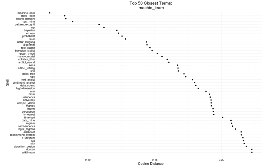
We also created the ability to review the distances between any word in the skill list and the 50 words closest to that word in the vector space. For example, here are the 50 closest skills to the skill “machin_learn”, which, of course, is the stemmed version of “machine learning”:
The full list of skills and the groups to which they were assigned, along with the R code used for this portion of the project, is available on github.
b. Hierarchical Clustering
To go a step further than k-means clustering, we can also apply an agglomerative hierarchical clustering algorithm to the group of skills, using the same word vectors. As in k-means, hierarchical clustering groups a set of observations based on some “distance”, but instead of fixing the number of groups from the outset, the procedure is to start with each observation as its own cluster and then successively combine these clusters based on some aggregate measure of the distance between them. The distance measure between clusters is not the same as the distance measure between individual observations as in k-means, and there actually a few different choices for how to implement this “linkage method” between clusters. For the present task, clustering word vectors based on job skills, we preferred the method of complete linkage, which considers the inter-cluster distance to be the greatest distance between any two individual observations in the clusters to be merged. This method was chosen here because it tends to disfavor forming clusters with only a few skills in them, which we would want to avoid because many categories of skills with very few members seems less useful than having fewer broad categories of skills.
The process of successively combining clusters to form larger clusters can be visualized in a tree like structure called a dendrogram. Typically, this dendrogram is “cut” at some height to create the actual clusters used for a particular application, but in this case we will use the whole dendrogram, shown here without labels.
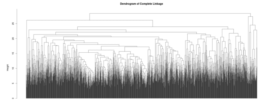
The results of this hierarchical clustering are not as easily interpretable when considering the dendrogram as a whole, but there are a few things additional things we can learn from this procedure. As mentioned in the analysis of the k-means clusters, some of the groups were much larger than others and could have been subdivided further. The same is true here, but in this case subdividing further just means cutting the dendrogram lower. While it is difficult to learn anything from the above image (even with labels), cutting at some reasonable value of height, say 20, will give a dendrogram with just 22 clusters, a number close to the 15 groups of skills used in the previous method.
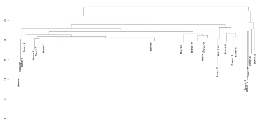
This is somewhat more manageable, and the labels for these clusters can be determined from looking at the sub dendrograms for any of these branches, such as branch 1, which apparently is a cluster of skills related to social media platforms.
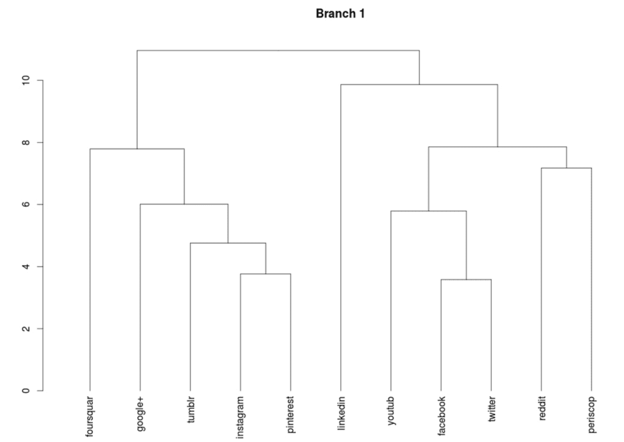
This sub-dendrogram is now somewhat more useful than the social media cluster found before because the sub grouping can easily be read off the diagram, such as how instagram and pinterest are treated as more similar, perhaps because they are more image oriented than the other platforms. Where this is particular useful is for those sub categories which are themselves a little too large to visualize directly in their own dendrogram, at which point we can cut again, and look at the sub-sub-dendrogram.
Aside from this advantage of having a clear method for further sub grouping, the other reason to use hierarchical clustering in addition to k-means is simply because it may give a different answer. Both methods require choices of input with no clear correct answer such as the number of clusters of the linkage method, so it shouldn’t be surprising if some skills are categorized differently in the two procedures. Using the dendrogram as a whole, we can come up with another measure of measuring “skill-relatedness” aside from just the word vector distance.
The dendrogram as a whole can be visualized in another way; as a matrix with the rows being the list of skills and the columns being the height of the dendrogram.
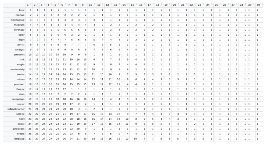
In this way the cells of the matrix show which categories the skills fall into at different heights on the dendrogram. Notice that towards the right of the table all of the categories eventually become “1”, as this is analogous to going to the top of the dendrogram where everything has been lumped into one category. To measure how closely related two skills are, we just have to find out the smallest column value for which two skills share the same category value. This gives us an additional feature, and in future applications where “skill-relatedness” may be useful, we can take a weighted average of these multiple measures of distance.
The script to generate these dendrograms, the full table, and the distance measure between skills is available on github.
III. LDA and Data Visualization
Our research also used a particular type of topic model known as Latent Dirichlet Allocation (LDA). This method will help us to discover topics within a collection of job descriptions.
The graph below is a screen shot of the interactive visualization of the LDA output derived from job descriptions. In general, we use a collection of job descriptions as a corpus, and skills as the terms we want to discover. Since each topic is defined by a probability distribution with support over many of word, it’s hard to interpret topics. So we created this interactive app to help us on topic interpretations. Each circle represents a topic. By hovering or clicking over a circle, you can see the most relevant terms for this topic.
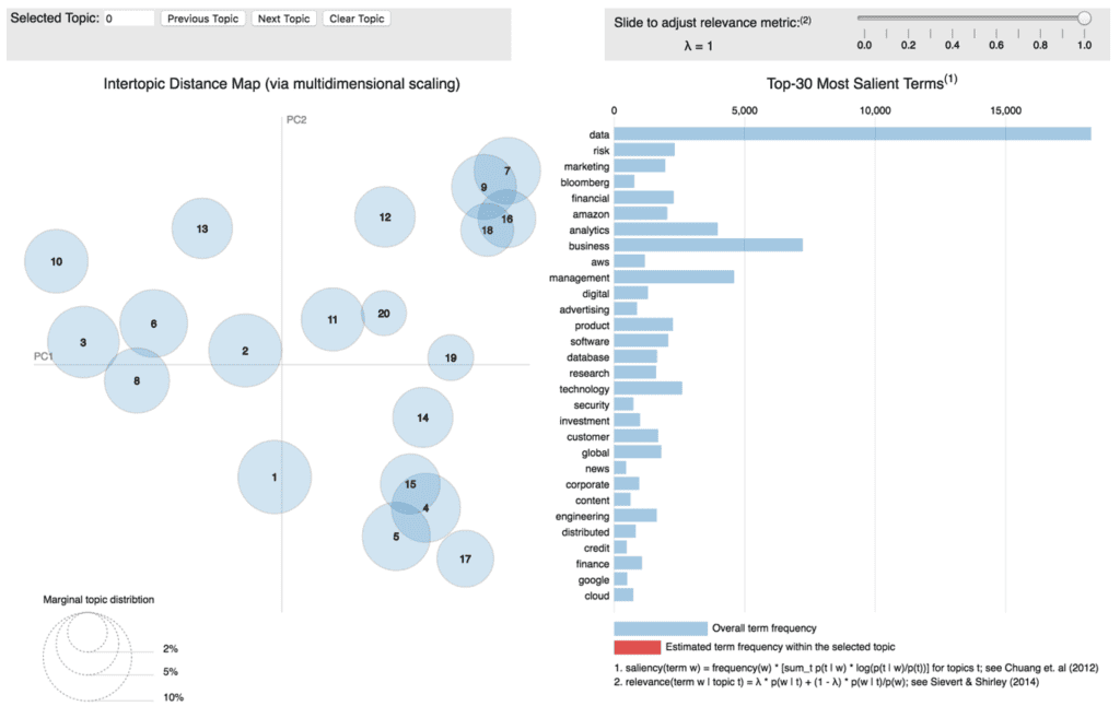
To see the relevance by terms, you can simply click on each term. For example, we can click on the term “data”, then the circles would change their size to show the relationship between “data” and the topics. The app shows that “data” is related to every topic, and it’s more important in topic 8, 9 and 11.
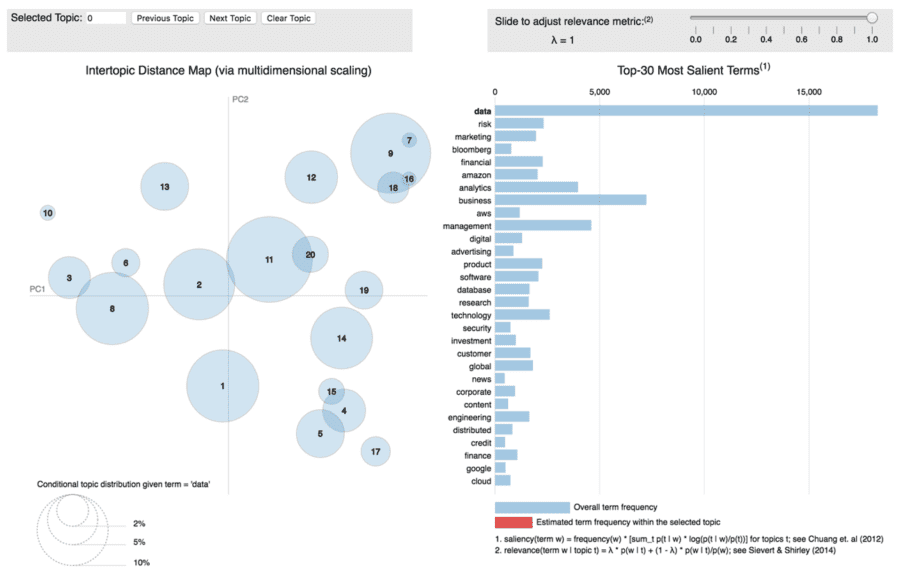
By way of example, in using this application we can find some interesting relationships:
- “Risk”, “Credit”, “Investments” and “Finance” share same topics (such as topic 9,7, 16 and 18). These topics are all in the upper-right area of PC1 and PC2
- “Data” and “Business” is everywhere
- “Amazon” and “Cloud” are a very important term in topic 10,13, 3 and 2; while “Google” and “Marketing” is highly related to topic15,4,5 and 17. This indicates Amazon is more related to cloud service and database, while Google’s products are popular in marketing.
Conclusion
Concerning the three approaches we took – word2vec with k-means clustering, word2vec with hierarchical clustering, and Latent Dirichlet Allocation – the obvious question to ask is which was “best” in measuring similarities in job skills. Because each of them was effective in assessing overall relatedness, to a large degree the answer depends on the application in which they’re used. For example, k-means is of linear complexity while hierarchical clustering runs in quadratic time, so the size of the data to be analyzed may become very important. Also, LDA was generally designed for comparisons of documents, versus the more “local” comparisons done on a word by word basis with word2vec. So LDA may be better if the application involves things like assessing which resumes or job descriptions are most similar (see also some interesting new research combining the benefits of word2vec and LDA). Other application requirements may highlight different differences between the approaches, and drive the algorithm choice.