

Neural network or artificial neural network is one of the frequently used buzzwords in analytics these days. Neural network is a machine learning technique which enables a computer to learn from the observational data. Neural network in computing is inspired by the way biological nervous system process information.
Biological neural networks consist of interconnected neurons with dendrites that receive inputs. Based on these inputs, they produce an output through an axon to another neuron.
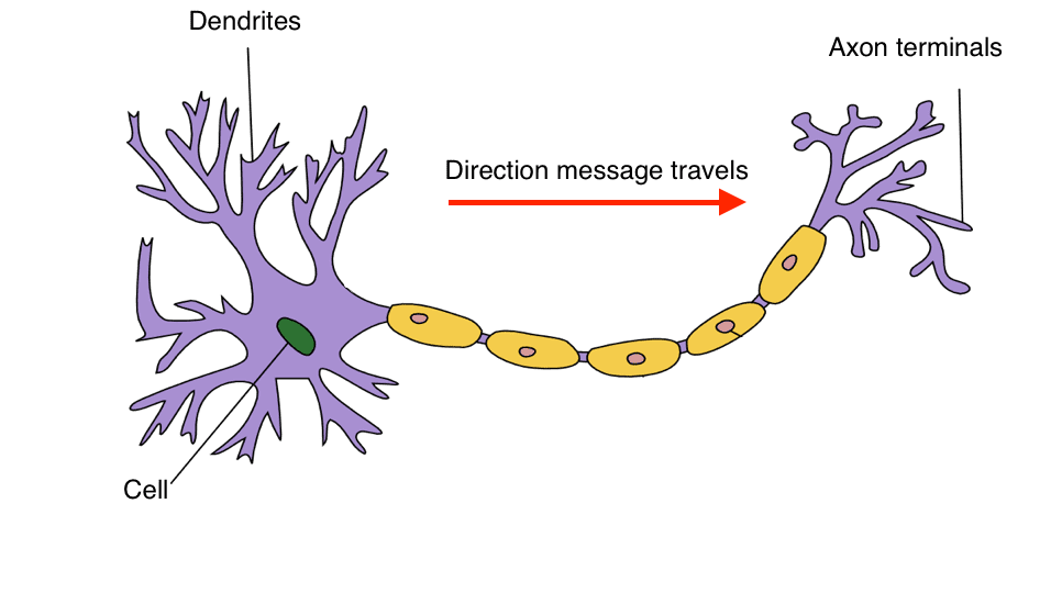
The term “neural network” is derived from the work of a neuroscientist, Warren S. McCulloch and Walter Pitts, a logician, who developed the first conceptual model of an artificial neural network. In their work, they describe the concept of a neuron, a single cell living in a network of cells that receives inputs, processes those inputs, and generates an output.
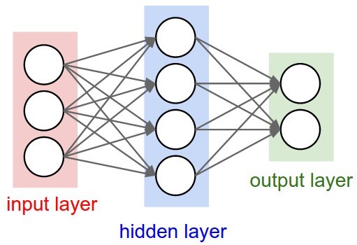
In the computing world, neural networks are organized on layers made up of interconnected nodes which contain an activation function. These patterns are presented to the network through the input layer which further communicates it to one or more hidden layers. The hidden layers perform all the processing and pass the outcome to the output layer.
Neural networks are typically used to derive meaning from complex and non-linear data, detect and extract patterns which cannot be noticed by the human brain. Here are some of the standard applications of neural network used these days.
- Pattern/ Image or object recognition
- Times series forecasting/ Classification
- Signal processing
- In self-driving cars to manage control
- Anomaly detection
These applications fall into different types of neural networks such as convolutional neural network, recurrent neural networks, and feed-forward neural networks. The first one is more used in image recognition as it uses a mathematical process known as convolution to analyze images in non-literal ways.
Let’s understand neural network in R with a dataset. The dataset consists of 724 observations and 7 variables.
“Companies.Changed” , “Experience.Score”, “Test.Score”, “Interview.Score”, “Qualification.Index”, “age”, “Status”
The following codes runs the network classifying ‘Status’ as a function of several independent varaibles. Status refers to recruitment with two variables: Selected and Rejected. To go ahead, we first need to install “neuralnet” package
>library(neuralnet)
>HRAnalytics<-read.csv(“filename.csv”)
> temp<-HRAnalytics
Now, removing NA from the data
> temp <-na.omit(temp)
> dim(temp) # 724 rows and 7 columns)
[1] 724 7
> y<-( temp$Status )
# Assigning levels in the Status Column
> levels(y)<-c(-1,+1)
> class(y)
[1] “factor”
# Now converting the factors into numeric
> y<-as.numeric (as.character (y))
> y <-as.data.frame(y)
> names(y)<-c(“Status”)
Removing the existing Status column and adding the new one Y
> temp$ Status <-NULL
> temp <-cbind(temp ,y)
> temp <-scale( temp )
> set.seed (100)
> n=nrow( temp )
The dataset will be split up in a subset used for training the neural network and another set used for testing. As the ordering of the dataset is completely random, we do not have to extract random rows and can just take the first x rows.
> train <- sample (1:n, 500, FALSE)
> f<- Status ~ Companies.Changed+Experience.Score+Test.Score+Interview.Score+Qualification.Index+age
Now we’ll build a neural network with 3 hidden nodes. We will Train the neural network with backpropagation. Backpropagation refers to the backward propagation of error.
> fit <- neuralnet (f, data = temp [train ,], hidden =3, algorithm = “rprop+”)
Plotting the neural network
> plot(fit, intercept = FALSE ,show.weights = TRUE)
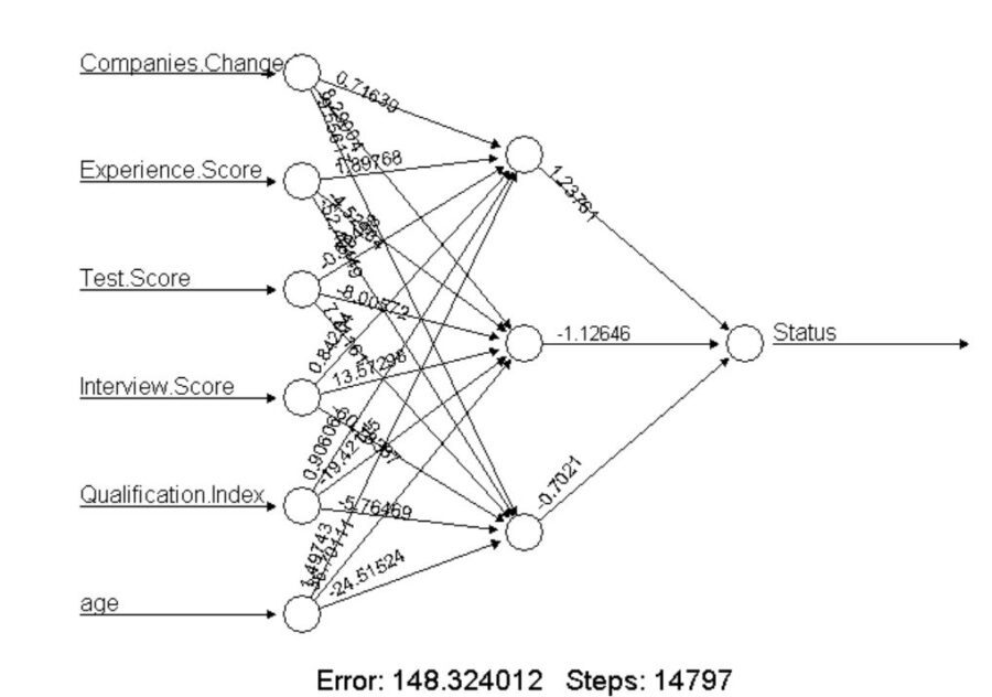
The above plot gives you an understanding of all the six input layers, three hidden layers, and the output layer.
> z<-temp
> z<-z[, -7]
The compute function is applied for computing the outputs based on the independent variables as inputs from the dataset.
Now, let’s predict on testdata (-train)
> pred <- compute (fit, z[-train,])
> sign(pred$net.result )
Now let’s create a simple confusion matrix:
> table(sign(pred$net.result),sign( temp[-train ,7]))
-1 1
-1 108 20
1 36 60
(108+60)/(108+20+36+60)
[1] 0.75
Here, the prediction accuracy is 75%
I hope the above example helped you understand how neural networks tune themselves to find the right answer on their own, increasing the accuracy of the predictions. Please note that the acceptable level of accuracy is considered to be over 80%. Unlike any other technique, neural networks also have certain limitations. One of the major limitation is that the data scientist or analyst has no other role than to feed the input and watch it train and gives the output. One of the article mentions that “with backpropagation, you almost don’t know what you’re doing”.
However, if we just ignore the negatives, the neural network has huge application and is a promising and practical form of machine learning. In the recent times, the best-performing artificial-intelligence systems in areas such as autonomous driving, speech recognition, computer vision, and automatic translation are all aided by neural networks. Only time will tell, how this field will emerge and offer intelligent solutions to problems we still have not thought of.