
In order to be a highly efficient, flexible, and production-ready library, TensorFlow uses dataflow graphs to represent computation in terms of the relationships between individual operations. Dataflow is a programming model widely used in parallel computing and, in a dataflow graph, the nodes represent units of computation while the edges represent the data consumed or produced by a computation unit.
This post is taken from the book Hands-On Neural Networks with TensorFlow 2.0 by Ekta Saraogi and Akshat Gupta. This book by Packt Publishing explains how TensorFlow works, from basics to advanced level with case-study based approach.
Representing computation using graphs comes with the advantage of being able to run the forward and backward passes required to train a parametric machine learning model via gradient descent, applying the chain rule to compute the gradient as a local process to every node; however, this is not the only advantage of using graphs.
Reducing the abstraction level and thinking about the implementation details of representing computation using graphs brings the following advantages:
- Parallelism: Using nodes to represent operations and edges that represent their dependencies, TensorFlow is able to identify operations that can be executed in parallel.
- Computation optimization: Being a graph, a well-known data structure, it is possible to analyze it with the aim of optimizing execution speed. For example, it is possible to detect unused nodes in the graph and remove them, hence optimizing it for size; it is also possible to detect redundant operations or sub-optimal graphs and replace them with the best alternatives.
- Portability: A graph is a language-neutral and platform-neutral representation of computation. TensorFlow uses Protocol Buffers(Protobuf), which is a simple language-neutral, platform-neutral, and extensible mechanism for serializing structured data to store graphs. This, in practice, means that a model defined in Python using TensorFlow can be saved in its language-neutral representation (Protobuf) and then used inside another program written in another language.
- Distributed execution: Every graph’s node can be placed on an independent device and on a different machine. TensorFlow will take care of the communication between the nodes and ensure that the execution of a graph is correct. Moreover, TensorFlow itself is able to partition a graph across multiple devices, knowing that certain operations perform better on certain devices.
The main structure – tf.Graph
Python simplifies the graph description phase since it even creates a graph without the need to explicitly define it; in fact, there are two different ways to define a graph:
- Implicit: Just define a graph using the *methods. If a graph is not explicitly defined, TensorFlow always defines a default tf.Graph, accessible by calling tf.get_default_graph. The implicit definition limits the expressive power of a TensorFlow application since it is constrained to using a single graph.
- Explicit: It is possible to explicitly define a computational graph and thus have more than one graph per application. This option has more expressive power, but is usually not needed since applications that need more than one graph are not common.
In order to explicitly define a graph, TensorFlow allows the creation of tf.Graph objects that, through the as_default method, create a context manager; every operation defined inside the context is placed inside the associated graph. In practice, a tf.Graph object defines a namespace for the tf.Operation objects it contains.
The second peculiarity of the tf.Graph structure is its graph collections. Every tf.Graph uses the collection mechanism to store metadata associated with the graph structure. A collection is uniquely identified by a key and its content is a list of objects/operations. The user does not usually need to worry about the existence of a collection since they are used by TensorFlow itself to correctly define a graph.
Graph definition – from tf.Operation to tf.Tensor
A dataflow graph is the representation of a computation where the nodes represent units of computation, and the edges represent the data consumed or produced by the computation.
In the context of tf.Graph, every API call defines tf.Operation (node) that can have multiple inputs and outputs tf.Tensor (edges). For instance, referring to our main example, when calling tf.constant([[1, 2], [3, 4]], dtype=tf.float32), a new node (tf.Operation) named Const is added to the default tf.Graph inherited from the context. This node returns a tf.Tensor (edge) named Const:0.
Since each node in a graph is unique, if there is already a node named Const in the graph (that is the default name given to all the constants), TensorFlow will make it unique by appending the suffix ‘_1’, ‘_2’, and so on to the name. If a name is not provided, as in our example, TensorFlow gives a default name to each operation added and adds the suffix to make them unique in this case too.
The output tf.Tensor has the same name as the associated tf.Operation, with the addition of the :ID suffix. The ID is a progressive number that indicates how many outputs the operation produces. In the case of tf.constant, the output is just a single tensor, therefore ID=0; but there can be operations with more than one output, and in this case, the suffixes :0, :1, and so on are added to the tf.Tensor name generated by the operation.
It is also possible to add a name scope prefix to all operations created within a context—a context defined by the tf.name_scope call. The default name scope prefix is a / delimited list of names of all the active tf.name_scope context managers. In order to guarantee the uniqueness of the operations defined within the scopes and the uniqueness of the scopes themselves, the same suffix appending rule used for tf.Operation holds.
The following code snippet shows how our baseline example can be wrapped into a separate graph, how a second independent graph can be created in the same Python script, and how we can change the node names, adding a prefix, using tf.name_scope. First, we import the TensorFlow library:
(tf1)
import tensorflow as tf
Then, we define two tf.Graph objects (the scoping system allows you to use multiple graphs easily):
g1 = tf.Graph()
g2 = tf.Graph()
with g1.as_default():
A = tf.constant([[1, 2], [3, 4]], dtype=tf.float32)
x = tf.constant([[0, 10], [0, 0.5]])
b = tf.constant([[1, -1]], dtype=tf.float32)
y = tf.add(tf.matmul(A, x), b, name=”result”)
with g2.as_default():
with tf.name_scope(“scope_a”):
x = tf.constant(1, name=”x”)
print(x)
with tf.name_scope(“scope_b”):
x = tf.constant(10, name=”x”)
print(x)
y = tf.constant(12)
z = x * y
Then, we define two summary writers. We need to use two different tf.summary.FileWriter objects to log two separate graphs.
writer = tf.summary.FileWriter(“log/two_graphs/g1”, g1)
writer = tf.summary.FileWriter(“log/two_graphs/g2”, g2)
writer.close()
Run the example and use TensorBoard to visualize the two graphs, using the left-hand column on TensorBoard to switch between “runs.”
Nodes with the same name, x in the example, can live together in the same graph, but they have to be under different scopes. In fact, being under different scopes makes the nodes completely independent and completely different objects. The node name, in fact, is not only the parameter name passed to the operation definition, but its full path, complete with all of the prefixes.
In fact, running the script, the output is as follows:
Tensor(“scope_a/x:0”, shape=(), dtype=int32)
Tensor(“scope_b/x:0”, shape=(), dtype=int32)
As we can see, the full names are different and we also have other information about the tensors produced. In general, every tensor has a name, a type, a rank, and a shape:
- The nameuniquely identifies the tensor in the computational graphs. Using name_scope, we can prefix tensor names, thus changing their full path. We can also specify the name using the name attribute of every tf.* API call.
- The typeis the data type of the tensor; for example, float32, tf.int8, and so on.
- The rank, in the TensorFlow world (this is different from the strictly mathematical definition), is just the number of dimensions of a tensor; for example, a scalar has rank 0, a vector has rank 1, a matrix has rank 2, and so on.
- The shapeis the number of elements in each dimension; for example, a scalar has rank 0 and an empty shape of (), a vector has rank 1 and a shape of (D0), a matrix has rank 2 and a shape of (D0, D1), and so on.
Being a C++ library, TensorFlow is strictly statically typed. This means that the type of every operation/tensor must be known at graph definition time. Moreover, this also means that it is not possible to execute an operation among incompatible types.
Looking closely at the baseline example, it is possible to see that both matrix multiplication and addition operations are performed on tensors with the same type, tf.float32. The tensors identified by the Python variables A and b have been defined, making the type clear in the operation definition, while tensor x has the same tf.float32 type; but in this case, it has been inferred by the Python bindings, which are able to look inside the constant value and infer the type to use when creating the operation.
Another peculiarity of Python bindings is their simplification in the definition of some common mathematical operations using operator overloading. The most common mathematical operations have their counterpart as tf.Operation; therefore, using operator overloading to simplify the graph definition is natural.
The following table shows the available operators overloaded in the TensorFlow Python API:
|
Python operator |
Operation name |
|
__neg__ |
unary - |
|
__abs__ |
abs() |
|
__invert__ |
unary ~ |
|
__add__ |
binary + |
|
__sub__ |
binary - |
|
__mul__ |
binary elementwise * |
|
__floordiv__ |
binary // |
|
__truediv__ |
binary / |
|
__mod__ |
binary % |
|
__pow__ |
binary ** |
|
__and__ |
binary & |
|
__or__ |
binary | |
|
__xor__ |
binary ^ |
|
__le__ |
binary /kbd> |
|
__lt__ |
binary <= |
|
__gt__ |
binary > |
|
__ge__ |
binary <= |
|
__matmul__ |
binary @ |
Operator overloading allows a faster graph definition and is completely equivalent to their tf.* API call (for example, using __add__ is the same as using the tf.add function). There is only one case in which it is beneficial to use the TensorFlow API call instead of the associated operator overload: when a name for the operation is needed.
Graph placement – tf.device
tf.device creates a context manager that matches a device. The function allows the user to request that all operations created within the context it creates are placed on the same device. The devices identified by tf.device are more than physical devices; in fact, it is capable of identifying devices such as remote servers, remote devices, remote workers, and different types of physical devices (GPUs, CPUs, and TPUs). It is required to follow a device specification to correctly instruct the framework to use the desired device. A device specification has the following form:
/job:<JOB_NAME>/task:<TASK_INDEX>/device:<DEVICE_TYPE>:<DEVICE_INDEX>
Broken down as follows:
- <JOB_NAME>is an alpha-numeric string that does not start with a number
- <DEVICE_TYPE>is a registered device type (such as GPU or CPU)
- <TASK_INDEX>is a non-negative integer representing the index of the task in the job named <JOB_NAME>
- <DEVICE_NAME>is a non-negative integer representing the index of the device; for example, /GPU:0 is the first GPU
There is no need to specify every part of a device specification. For example, when running a single-machine configuration with a single GPU, you might use tf.device to pin some operations to the CPU and GPU.
We can thus extend our baseline example to place the operations on the device we choose. Thus, it is possible to place the matrix multiplication on the GPU, since it is hardware optimized for this kind of operation, while keeping all the other operations on the CPU.
Please note that since this is only a graph description, there's no need to physically have a GPU or to use the tensorflow-gpu package. First, we import the TensorFlow library:
(tf1)
import tensorflow as tf
Now, use the context manager to place operations on different devices, first, on the first CPU of the local machine:
with tf.device("/CPU:0"):
A = tf.constant([[1, 2], [3, 4]], dtype=tf.float32)
x = tf.constant([[0, 10], [0, 0.5]])
b = tf.constant([[1, -1]], dtype=tf.float32)
Then, on the first GPU of the local machine:
with tf.device("/GPU:0"):
mul = A @ x
When the device is not forced by a scope, TensorFlow decides which device is better to place the operation on:
y = mul + b
Then, we define the summary writer:
writer = tf.summary.FileWriter("log/matmul_optimized", tf.get_default_graph())
writer.close()
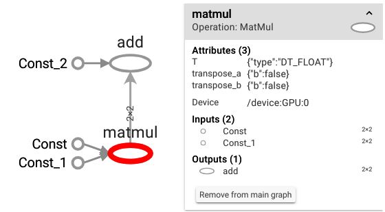
If we look at the generated graph, we'll see that it is identical to the one generated by the baseline example, with two main differences:
- Instead of having a meaningful name for the output tensor, we have just the default one
- Clicking on the matrix multiplication node, it is possible to see (in TensorBoard) that this operation must be executed in the first GPU of the local machine
The matmul node is placed on the first GPU of the local machine, while any other operation is executed in the CPU. TensorFlow takes care of communication among different devices in a transparent manner:
Graph execution – tf.Session
tf.Session is a class that TensorFlow provides to represent a connection between the Python program and the C++ runtime.
The tf.Session object is the only object able to communicate directly with the hardware (through the C++ runtime), placing operations on the specified devices, using the local and distributed TensorFlow runtime, with the goal of concretely building the defined graph. The tf.Session object is highly optimized and, once correctly built, caches tf.Graph in order to speed up its execution.
Being the owner of physical resources, the tf.Session object must be used as a file descriptor to do the following:
- Acquire the resources by creating a Session(the equivalent of the open operating system call)
- Use the resources (the equivalent of using the read/write operation on the file descriptor)
- Release the resources with tf.Session.close(the equivalent of the close call)
Typically, instead of manually defining a session and taking care of its creation and destruction, a session is used through a context manager that automatically closes the session at the block exit.
The constructor of tf.Session is fairly complex and highly customizable since it is used to configure and create the execution of the computational graph.
In the simplest and most common scenario, we just want to use the current local hardware to execute the previously described computational graph as follows:
(tf1)
# The context manager opens the session
with tf.Session() as sess:
# Use the session to execute operations
sess.run(...)
# Out of the context, the session is closed and the resources released
There are more complex scenarios in which we wouldn't want to use the local execution engine, but use a remote TensorFlow server that gives access to all the devices it controls. This is possible by specifying the target parameter of tf.Session just by using the URL (grpc://) of the server:
(tf1)
# the IP and port of the TensorFlow server
ip = "192.168.1.90"
port = 9877
with tf.Session(f"grpc://{ip}:{port}") as sess:
sess.run(...)
By default, the tf.Session will capture and use the default tf.Graph object, but when working with multiple graphs, it is possible to specify which graph to use by using the graph parameter. It's easy to understand why working with multiple graphs is unusual, since even the tf.Session object is able to work with only a single graph at a time.
The third and last parameter of the tf.Session object is the hardware/network configuration specified through the config parameter. The configuration is specified through the tf.ConfigProto object, which is able to control the behavior of the session. The tf.ConfigProto object is fairly complex and rich with options, the most common and widely used being the following two (all the others are options used in distributed, complex environments):
- allow_soft_placement: If set to True, it enables a soft device placement. Not every operation can be placed indifferently on the CPU and GPU, because the GPU implementation of the operation may be missing, for example, and using this option allows TensorFlow to ignore the device specification made via deviceand place the operation on the correct device when an unsupported device is specified at graph definition time.
- gpu_options.allow_growth: If set to True, it changes the TensorFlow GPU memory allocator; the default allocator allocates all the available GPU memory as soon as the tf.Sessionis created, while the allocator used when allow_growth is True gradually increases the amount of memory allocated. The default allocator works in this way because, in production environments, the physical resources are completely dedicated to the tf.Session execution, while, in a standard research environment, the resources are usually shared (the GPU is a resource that can be used by other processes while the TensorFlow tf.Session is in execution).
The baseline example can now be extended to not only define a graph, but to proceed on to an effective construction and the execution of it:
import tensorflow as tf
import numpy as np
A = tf.constant([[1, 2], [3, 4]], dtype=tf.float32)
x = tf.constant([[0, 10], [0, 0.5]])
b = tf.constant([[1, -1]], dtype=tf.float32)
y = tf.add(tf.matmul(A, x), b, name="result")
writer = tf.summary.FileWriter("log/matmul", tf.get_default_graph())
writer.close()
with tf.Session() as sess:
A_value, x_value, b_value = sess.run([A, x, b])
y_value = sess.run(y)
# Overwrite
y_new = sess.run(y, feed_dict={b: np.zeros((1, 2))})
print(f"A: {A_value}\nx: {x_value}\nb: {b_value}\n\ny: {y_value}")
print(f"y_new: {y_new}")
The first sess.run call evaluates the three tf.Tensor objects, A, x, b, and returns their values as numpy arrays.
The second call, sess.run(y), works in the following way:
- yis an output node of an operation: backtrack to its inputs
- Recursively backtrack through every node until all the nodes without a parent are found
- Evaluate the input; in this case, the A, x, btensors
- Follow the dependency graph: the multiplication operation must be executed before the addition of its result with b
- Execute the matrix multiplication
- Execute the addition
The addition is the entry point of the graph resolution (Python variable y) and the computation ends.
The first print call, therefore, produces the following output:
A: [[1. 2.]
[3. 4.]]
x: [[ 0. 10. ]
[ 0. 0.5]]
b: [[ 1. -1.]]
y: [[ 1. 10.]
[ 1. 31.]]
The third sess.run call shows how it is possible to inject into the computational graph values from the outside, as numpy arrays, overwriting a node. The feed_dict parameter allows you to do this: usually, inputs are passed to the graph using the feed_dict parameter and through the overwriting of the tf.placeholder operation created exactly for this purpose.
tf.placeholder is just a placeholder created with the aim of throwing an error when values from the outside are not injected inside the graph. However, the feed_dict parameter is more than just a way to feed the placeholders. In fact, the preceding example shows how it can be used to overwrite any node. The result produced by the overwriting of the node identified by the Python variable, b, with a numpy array that must be compatible, in terms of both type and shape, with the overwritten variable, is as follows:
y_new: [[ 0. 11.]
[ 0. 32.]]
The baseline example has been updated in order to show the following:
- How to build a graph
- How to save a graphical representation of the graph
- How to create a session and execute the defined graph
So far, we have used graphs with constant values and used the feed_dict parameter of the sess.run call to overwrite a node parameter. However, since TensorFlow is designed to solve complex problems, the concept of tf.Variable has been introduced: every parametric machine learning model can be defined and trained with TensorFlow.
In this post we talked about how dataflow graphs work in TensorFlow. To know, the implementation of convolution neural network in TensorFlow for via Churn Prediction Case Study and pneumonia detection from the x-ray case study, read the book Hands-On Neural Networks with TensorFlow 2.0 by Packt Publishing.