
It is always hard to find a proper model to forecast time series data. One of the reasons is that models that use time-series data often expose to serial correlation. In this article, we will compare k nearest neighbor (KNN) regression which is a supervised machine learning method, with a more classical and stochastic process, autoregressive integrated moving average (ARIMA).
We will use the monthly prices of refined gold futures(XAUTRY) for one gram in Turkish Lira traded on BIST(Istanbul Stock Exchange) for forecasting. We created the data frame starting from 2013. You can download the relevant excel file from here.
#building the time series datalibrary(readxl)df_xautry <- read_excel("xau_try.xlsx")xautry_ts <- ts(df_xautry$price,start = c(2013,1),frequency = 12)KNN Regression
We are going to use tsfknn package which can be used to forecast time series in R programming language. KNN regression process consists of instance, features, and targets components. Below is an example to understand the components and the process.
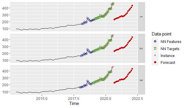
library(tsfknn)pred <- knn_forecasting(xautry_ts, h = 6, lags = 1:12,k=3)autoplot(pred, highlight = "neighbors",faceting = TRUE)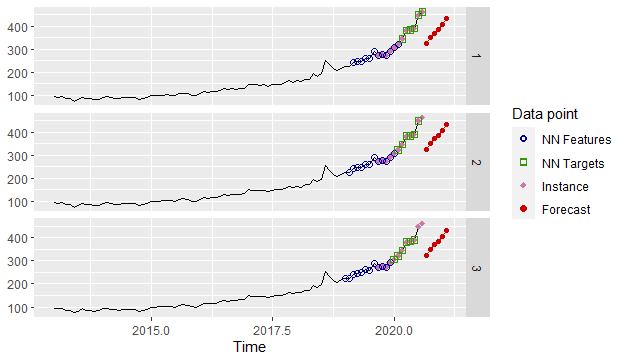
The lags parameter indicates the lagged values of the time series data. The lagged values are used as features or explanatory variables. In this example, because our time series data is monthly, we set the parameters to 1:12. The last 12 observations of the data build the instance, which is shown by purple points on the graph.
This instance is used as a reference vector to find features that are the closest vectors to that instance. The relevant distance metric is calculated by the Euclidean formula as shown below:
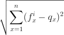
 denotes the instance and
  indicates the features that are ranked in order by the distance metric. The k parameter determines the number of k closest features vectors which are called k nearest neighbors.
nearest_neighbors function shows the instance, k nearest neighbors, and the targets.
nearest_neighbors(pred)#$instance#Lag 12 Lag 11 Lag 10 Lag 9 Lag 8 Lag 7 Lag 6 Lag 5 Lag 4 Lag 3 Lag 2#272.79 277.55 272.91 291.12 306.76 322.53 345.28 382.02 384.06 389.36 448.28# Lag 1#462.59#$nneighbors# Lag 12 Lag 11 Lag 10 Lag 9 Lag 8 Lag 7 Lag 6 Lag 5 Lag 4 Lag 3 Lag 2#1 240.87 245.78 248.24 260.94 258.68 288.16 272.79 277.55 272.91 291.12 306.76#2 225.74 240.87 245.78 248.24 260.94 258.68 288.16 272.79 277.55 272.91 291.12#3 223.97 225.74 240.87 245.78 248.24 260.94 258.68 288.16 272.79 277.55 272.91# Lag 1 H1 H2 H3 H4 H5 H6#1 322.53 345.28 382.02 384.06 389.36 448.28 462.59#2 306.76 322.53 345.28 382.02 384.06 389.36 448.28#3 291.12 306.76 322.53 345.28 382.02 384.06 389.36Targets are the time-series data that come right after the nearest neighbors and their number is the value of the h parameter. The targets of the nearest neighbors are averaged to forecast the future h periods.

As you can see from the above plotting, features or targets might overlap the instance. This is because the time series data has no seasonality and is in a specific uptrend. This process we mentioned so far is called MIMO(multiple-input-multiple-output) strategy that is a forecasting method used as a default with KNN.
Decomposing and analyzing the time series data
Before we mention the model, we first analyze the time series data on whether there is seasonality. The decomposition analysis is used to calculate the strength of seasonality which is described as shown below:
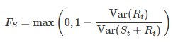
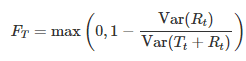
#Seasonality and trend measurementslibrary(fpp2)fit <- stl(xautry_ts,s.window = "periodic",t.window = 13,robust = TRUE)seasonality <- fit %>% seasonal()trend <- fit %>% trendcycle()remain <- fit %>% remainder()#Trend1-var(remain)/var(trend+remain)#[1] 0.990609#Seasonality1-var(remain)/var(seasonality+remain)#[1] 0.2624522The stl function is a decomposing time series method. STL is short for seasonal and trend decomposition using loess, which loess is a method for estimating nonlinear relationships. The t.window(trend window) is the number of consecutive observations to be used for estimating the trend and should be odd numbers. The s.window(seasonal window) is the number of consecutive years to estimate each value in the seasonal component, and in this example, is set to ‘periodic‘ to be the same for all years. The robust parameter is set to ‘TRUE‘ which means that the outliers won’t affect the estimations of trend and seasonal components.
When we examine the results from the above code chunk, it is seen that there is a strong uptrend with 0.99, weak seasonality strength with 0.26, because that any value less than 0.4 is accepted as a negligible seasonal effect. Because of that, we will prefer the non-seasonal ARIMA model.
Non-seasonal ARIMA
This model consists of differencing with autoregression and moving average. Let’s explain each part of the model.
Differencing: First of all, we have to explain stationary data. If data doesn’t contain information pattern like trend or seasonality in other words is white noise that data is stationary. White noise time series has no autocorrelation at all.
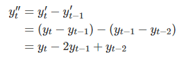
Differencing is a simple arithmetic operation that extracts the difference between two consecutive observations to make that data stationary.
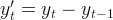
The above equation shows the first differences that difference at lag 1. Sometimes, the first difference is not enough to obtain stationary data, hence, we might have to do differencing of the time series data one more time(second-order differencing).
In autoregressive models, our target variable is a linear combination of its own lagged variables. This means the explanatory variables of the target variable are past values of that target variable. The AR(p) notation denotes the autoregressive model of order p and the  denotes the white noise.

Moving average models, unlike autoregressive models, they use past error(white noise) values for predictor variables. The MA(q) notation denotes the autoregressive model of order q.

If we integrate differencing with autoregression and the moving average model, we obtain a non-seasonal ARIMA model which is short for the autoregressive integrated moving average.

 is the differenced data and we must remember it may have been first and second order. The explanatory variables are both lagged values of
  and past forecast errors. This is denoted as ARIMA(p,d,q) where p; the order of the autoregressive; d, degree of first differencing; q, the order of the moving average.
Modeling with non-seasonal ARIMA
Before we model the data, first we split the data as train and test to calculate accuracy for the ARIMA model.
#Splitting time series into training and test datatest <- window(xautry_ts, start=c(2019,3))train <- window(xautry_ts, end=c(2019,2)) |
#ARIMA modelinglibrary(fpp2)fit_arima<- auto.arima(train, seasonal=FALSE, stepwise=FALSE, approximation=FALSE)fit_arima#Series: train#ARIMA(0,1,2) with drift#Coefficients:# ma1 ma2 drift# -0.1539 -0.2407 1.8378#s.e. 0.1129 0.1063 0.6554#sigma^2 estimated as 86.5: log likelihood=-264.93#AIC=537.85 AICc=538.44 BIC=547.01 |
As seen above code chunk, stepwise=FALSE, approximation=FALSE parameters are used to amplify the searching for all possible model options. The drift component indicates the constant c which is the average change in the historical data. From the results above, we can see that there is no autoregressive part of the model, but a second-order moving average with the first differencing.
Modeling with KNN
#Modeling and forecastinglibrary(tsfknn)pred <- knn_forecasting(xautry_ts, h = 18, lags = 1:12,k=3) |
#Forecasting plotting for KNNautoplot(pred, highlight = "neighbors", faceting = TRUE) |
Forecasting and accuracy comparison between the models
#ARIMA accuracyf_arima<- fit_arima %>% forecast(h =18) %>% accuracy(test)f_arima[,c("RMSE","MAE","MAPE")]# RMSE MAE MAPE #Training set 9.045488 5.529203 4.283023#Test set 94.788638 74.322505 20.878096 |
For forecasting accuracy, we take the results of the test set shown above.
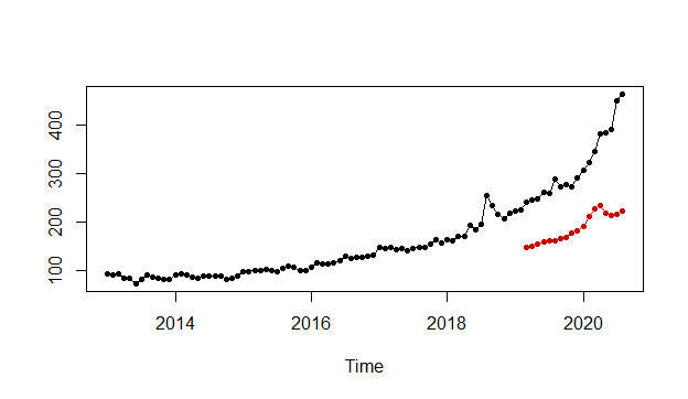
#Forecasting plot for ARIMAfit_arima %>% forecast(h=18) %>% autoplot()+ autolayer(test)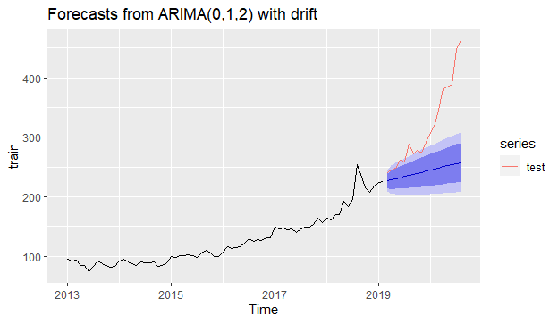
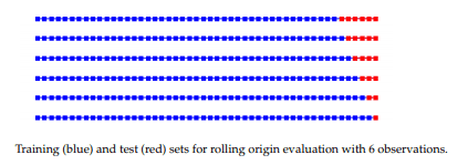
#KNN Accuracyro <- rolling_origin(pred, h = 18,rolling = FALSE)ro$global_accu# RMSE MAE MAPE#137.12465 129.77352 40.22795The rolling_origin function is used to evaluate the accuracy based on rolling origin. The rolling parameter should be set to FALSE which makes the last 18 observations as the test set and the remaining as the training set; just like we did for ARIMA modeling before. The test set would not be a constant vector if we had set the rolling parameter to its default value of TRUE. Below, there is an example for h=6 that rolling_origin parameter set to TRUE. You can see the test set dynamically changed from 6 to 1 and they eventually build as a matrix, not a constant vector.
#Accuracy plot for KNNplot(ro) |
When we compare the results of the accuracy measurements like RMSE or MAPE, we can easily see that the ARIMA model is much better than the KNN model for our non-seasonal time series data.
The original article is here.
References
- Forecasting: Principles and Practice, Rob J Hyndman and George Athanasopoulos
- Time Series Forecasting with KNN in R: the tsfknn Package, Francisco Martínez, María P. Frías, Francisco Charte, and Antonio J. Rivera
- Autoregression as a means of assessing the strength of seasonality …Rahim Moineddin, Ross EG Upshur, Eric Crighton & Muhammad Mamdani