
In my prior blog post, I wrote of a clever elf that could predict the outcome of a mathematically fair process roughly ninety percent of the time. Actually, it is ninety-three percent of the time and why it is ninety-three percent instead of ninety percent is also important.
The purpose of the prior blog post was to illustrate the weakness of using the minimum variance unbiased estimator (MVUE) in applied finance. Nonetheless, that begs a more general question of when and why it should be used, or a Bayesian or Likelihood-based method should be applied. Fortunately, the prior blog post provides a way of looking at the problem.
Fisher’s Likelihood-based, Pearson and Neyman’s Frequency-based and Laplace’s method of inverse probability really are at odds with one another. Indeed, much of the literature of the mid-twentieth century had a polemical ring to it. Unfortunately, what ended up coming about was a hybridization of the tools, and so it can be challenging to see how the differing properties matter.
In fact, each type of tool was created to solve different kinds of problems. It should be unsurprising that they excel in some places and may even be problematic in some cases.
In the prior blog post, the clever elf was able to have perfect knowledge of the outcome of a mathematically fair process in eighty percent of the cases and was superior in thirteen of the remaining twenty percent of the cases because the MVUE violates the likelihood principle. Of course, that is by design. It is supposed to violate the likelihood principle. It could not display its virtues if it tried to conform. Nonetheless, it forces a split between Pearson and Neyman on one side and Fisher and Laplace on the other.
In most statistical disagreements, the split is among methods built around null hypothesis methods and Bayesian methods. In this case, Fisher’s method will sit on Laplace’s side of the fence rather than Pearson and Neyman’s. The goal of this post is neither to defend nor to attack the likelihood principle. Others have done that with great technical skill.
This post is to provide a background of the issues separate from a technical presentation of it. While this post could muck around in measure theory, the goal is to extend the example of the cakes so the differences can be made apparent. As it happens, there is a clean and clear break in the information used between the methodologies.
The likelihood principle is divisive in the field of probability and statistics. Some adherents to the principle argue that it rules out Pearson and Neyman’s methodology entirely. Opponents either say that its construction is flawed in some way or, simply state that for most practical problems, no one need care about the difference because orthodox procedures work often enough in practical situations. Yet these positions illustrate why not knowing the core arguments could cause a data scientist or subject matter expert to choose the wrong method.
The likelihood principle follows from two separate tenets that are not individually controversial or at least not very controversial. There has been work to explore it, such as by Berger and Wolpert. There has also been work to refute it and to refute the refutations. See, for example, Deborah Mayo’s work. So far, no one has generated an argument so convincing that the opposing sides believe that the discussion is even close to being closed. It remains a fertile field for graduate students to produce research and advancements.
The first element of the likelihood principle is the sufficiency principle. No one tends to dispute it. The second is the conditionality principle. It tends to be the source of any contention. We will only consider the discrete case here, but for a discussion of the continuous case, see Berger and Wolpert’s work on it listed below.
A little informally, the weak conditionality principle supposes that two possible experiments could take place regarding a parameter. In Birnbaum’s original formulation, he considered two possible experiments that could be chosen, each with a probability of one-half. The conditionality principle states that all of the evidence regarding the parameter comes only from the experiment that was actually performed. The experiment that did not happen plays no role. That last sentence is the source of the controversy.
Imagine that a representative sample is chosen from a population to measure the heights of members. There will be several experiments performed by two research groups for many different studies over many unrelated topics.
The lab has two types of equipment that can be used. The first is a carpenter’s tape that is accurate to 1/8th of an inch (3.125 mm), while the other is a carpenter’s tape that is accurate to 1 millimeter. A coin is tossed to determine which team gets which carpenter’s tape.
The conditionality principle states that the results of the experiment only depend on the accuracy of the instrument used and the members of the sample and that the information that would have been collected by using the other device or a different sample has to be ignored. To most people, that would be obvious, but that is the controversial part.
Pearson and Neyman’s methods choose the optimal solution before seeing any data. Any randomness that impacts the process must be accounted for, and so the results that could have been obtained but were not are supposed to affect the form of the solution.
Pearson and Neyman’s algorithm is optimal, having never seen the data, but may not be optimal after seeing the data. There can exist an element of the sample space that would cause Pearson and Neyman’s method to produce poor results. The guarantee is for good average results upon repetition over the sample space, not good results in any one experiment.
There are examples of pathological results in the literature where a Frequentist and a Bayesian statistician can draw radically different solutions with the same data. To understand another place that a violation of the likelihood principle may occur, consider the lowly t-test.
Imagine a more straightforward case where the lab only had one piece of equipment, and it was accurate to 1 millimeter. If a result is significant, then the sample statistic is as extreme or more extreme than what one would expect if the null is true. It compares the result to the set of all possible samples that could have been taken if the null is true.
Of course, more extreme values were not observed for the sample mean. If a more extreme result were found, then that would have been the result and not the one actually observed. What if the result is the most extreme result any person has ever seen, can someone really argue that the tail probability is full?
The conditionality principle says that if you didn’t see it, then you do not have information about it. You cannot use samples that were not seen to perform inference. That excludes all t-, F-, z-tests, and most Frequentist tests because they are conditioned on a model that assumes that certain things are real that have never been observed.
A big difference between Laplace and Fisher on one side and Pearson and Neyman on the other is whether all the evidence that you have about a parameter is in the sample, or whether samples unseen must be included as well.
The non-controversial part of the likelihood principle is the sufficiency principle. The sufficiency principle is a core element of all methods. It states something pretty obvious.
Imagine you are performing a set of experiments to gather evidence about some parameter, and you are going to use a statistic  , where t is a statistic sufficient for the parameter. Then if you conducted two experiments and the statistics were equal,
  , then the evidence about the parameter in both experiments is equal.
When the two principles are combined, Birnbaum asserts that the likelihood principle follows from it. The math lands on the following proposition. If you are performing an experiment, then the evidence about a parameter should depend only on the experiment actually conducted and the data observed through the likelihood function.
In other words, Fisher’s likelihood function and Laplace’s Likelihood function are the only functions that contain all the information from the experiment. If you do not use the method of maximum likelihood or the method of inverse probability, then you are not using all of the information. You are surrendering information if you choose something else.
Before we look at the ghostly cakes again, there are two reasons to rule out Fisher’s method of maximum likelihood. The first is that, as mentioned in the prior blog post, there is not a unique maximum likelihood estimator in this case. The second, however, is that Fisher’s method isn’t designed so that you could make a decision from knowing its value. It is designed for epistemological inference. The p-value does not imply that there is an action that would follow from knowing it. It is designed to provide knowledge, not to prescribe actions or behaviors.
If you use Fisher’s method as he intended, then the p-value is the weight of the evidence against your idea. It doesn’t have an alternate hypothesis or an automatic cut-off. Either you decide that the weight is enough that you should further investigate the phenomenon, or it isn’t enough, and you go on with life investigating other things.
In the prior blog post, the engineer was attempting to find the center of the cake using Cartesian coordinates. The purpose was to take an action that is cutting a cake through a particular point.
She had a blade that was long enough regardless of where the cake sat that was anchored in the origin. In practice, her only real concern was the angle, but not the distance. Even though two Cartesian dimensions were measured, only one is used in polar coordinates, the angle.
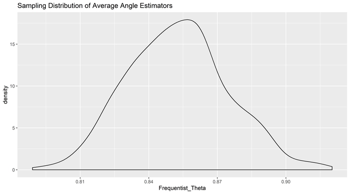
The clever elf, however, was using a Bayesian method, and the likelihood was based on the distance between points as well as the angles. As such, it had to use both dimensions to get a result. The reason the MVUE was less precise is that it violates the likelihood principle and throws away information.
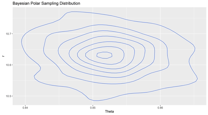
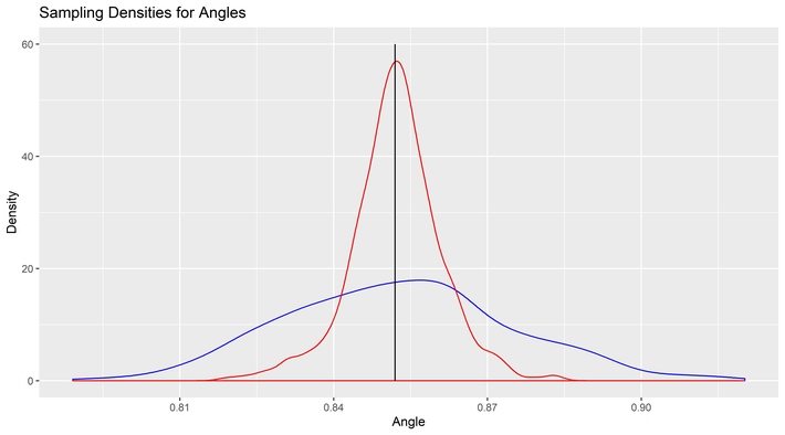
It is here we can take another look at our ghostly cakes by leaving the Cartesian coordinate system and moving over to polar coordinates so we can see the source of the information loss directly. This difference can be seen in the sampling distribution of the two tools by angle.
Why bother with the MVUE at all? After all, when it doesn’t match Fisher’s method of maximum likelihood, then it must be a method of mediocre likelihood. What does the MVUE have to offer that the Bayesian posterior density cannot
The MVUE is an estimator that comes with an insurance policy. It also permits answers to questions that the Bayesian posterior cannot answer.
Neither Laplace’s Bayesian nor Fisher’s Likelihood methods directly concern themselves with either precision or accuracy. Both tend to be biased methods, but that is in part because neither method cares about bias. An unbiased estimator solves a type of problem that a biased estimator cannot solve.
Imagine an infinite number of parallel universes where each is slightly different. A method is either unbiased and accurate or biased and inaccurate. For someone trying to determine which world they live in, the use of a Bayesian method implies they will always tend to believe they live in one of the nearby universes, but never find which one is their own, except by chance.
Using Pearson and Neyman’s method also allows a guarantee against the frequency of false positives and a way to control for false negatives. Such assurance can be valuable, particularly in manufacturing quality control. That assurance extends to confidence, tolerance, and predictive intervals. Such a guarantee of coverage also holds value in academia.
Finally, under mild circumstances such as correct instrumentation and methodology, Pearson and Neyman’s method allows for a solution to inferences in two ways that are unavailable to the Bayesian approach.
First, Frequency methods allow for a complete form of reasoning that is not generally available to Bayesian methods. Bayesian methods lack a null hypothesis and are not restricted to two hypotheses. There should be one hypothesis for every possible combination of ways the world could exist. Unfortunately, it is possible that the set of Bayesian hypotheses cannot contain the real model of the world.
Before Einstein and relativity, there couldn’t have been a hypothesis that included curvatures in space-time and so a Bayesian test would have found the closest fit to reality but also would have been wrong. Without knowing about relativity, a null hypothesis could test whether Newton’s laws were valid for the orbit of Mercury and discover that they were not. That does not mean a good solution exists from current knowledge, but it would show that there is something wrong with Newton’s laws.
Additionally, Bayesian methods have no good solution to solve a sharp null hypothesis. A null hypothesis is sharp if it is of the form  . Although there is a Bayesian solution in the discrete case, in the continuous case, there cannot be one because it would have zero measure. If it is assumed that
  , then the world should work in a specific manner. If that is the real question, then a Bayesian solution cannot provide a really good solution. There are Bayesian approximations but no exact answer.
In applied finance, only Bayesian methods make sense for data scientists and subject matter experts, but in academic finance, there is a strong argument for Frequentist methods. The insurance policy is paid for in information loss, but it provides benefits unavailable to other methods.
If the engineer in the prior blog post had been using polar coordinates rather than Cartesian coordinates, there would not be a need to measure the distance from the origin to find the MVUE because the blade was built to be long enough. The Bayesian method would have required the measurement of the distance from the origin.
At a certain level, it seems strange that adding any variable to the angles observed could improve the information about the angle alone, yet it does. The difference between the MVUE and the posterior mean is obvious. The likelihood function requires knowledge of the distances. Even though the distance estimator is not used in the cutting of the cake, and even though there are errors in the estimation of the distance to the center from each point, the increase in information substantially outweighs the added source of error. Overall, the noise gets reduced from the added information.
Finally, the informational differences should act as a warning to model builders. Information that can be discarded using a Frequency-based model may be critical information in a Bayesian model. Models like the CAPM come apart in a Bayesian construction, implying that a different approach is required by the subject matter expert. The data scientist performing the implementation will have differences too.
Models of finance tend to be generic and have a cookbook feel. That is because the decision-tree implicit in financial modeling is around finding the right tool for the right mix of general issues. Concerns for things such as heteroskedasticity, autocorrelation, or other symptoms or pathologies all but vanish in a Bayesian methodology. Instead, the headaches often revolve around combinatorics, finding local extreme values, and the data generation process. To take advantage of all available information, the model has to contain it. In the ghostly cakes, more than the angle is necessary. The model needs to be proposed and measured.
Berger, J. O., & Wolpert, R. L. (1984). The likelihood principle. Hayward, Calif: Institute of Mathematical Statistics.
Mayo, Deborah G. (2014) On the Birnbaum Argument for the Strong Likelihood Principle. Statist. Sci. 29, no. 2, 227-239