
In the statistical literature, for ordinal types of data, are known lots of indicators to measure the degree of the polarization phenomenon. Typically, many of the widely used measures of distributional variability are defined as a function of a reference point, which in some “sense” could be considered representative for the entire population. This function indicates how much all the values differ from the point that is considered “typical”.
Of all measures of variability, the variance is a well-known example that use the mean as a reference point. However, mean-based measures depend to the scale applied to the categories (Allison & Foster, 2004) and are highly sensitive to outliers. An alternative approach is to compare the distribution of an ordinal variable with that of a maximum dispersion, that is the two-point extreme distribution (i.e A distribution in which half of the population is concentrated in the lowest category and half in the top category). Using this procedure, three measures of variation for ordinal categorical data have been suggested, the Linear Order of Variation – LOV (Berry & Mielke, 1992), the Index Order of Variation – IOV (Leik, 1966) and the COV (Kvalseth, Coefficients of variations for nominal and ordinal catego…). All these indices are based on the cumulative relative frequency distribution (CDF), since this contains all the distributional information of any ordinal variable (Blair & Lacy, 1996). Consequently, none of these measures rely on ordinal assumptions about distances between categories.
At this point, the reader might wonder if this approach to dispersion is adequate to define the functional form of a polarization measure. “Why not measure the dispersion of the observed distribution as the distance from a point of minimal dispersion?”. This question has been addressed by Blair and Lacy in the article Statistics of ordinal variation (Blair & Lacy, 2000). They argue that this approach is impractical since there are as many one-point distribution as the number of categories. Therefore, it would not be clear, from which one we should calculate the distance.
Then, is there another way to compare the dispersion of a distribution that does not depend on its location? Is the space of the cumulative frequency vector the only way to represent all possible distributions?
To address this challenge, I propose a new representation of probability measures, the Bilateral Cumulative Distribution Function (BCDF), which derives from a generalization of the CDF. Basically, it is an extended CDF that can be easily obtained by folding its upper part, commonly known as survival function or complementary CDF. Unlike the CDF, this functional has a finite constant area independently of the probability distribution (pdf) and, therefore, more convenient for any distribution comparison. For the definition, properties and computation of the BCDF see Appendix A3:(Pinzari et all 2019)
On this basis, to capture the amount of fluctuations about the mean and simultaneously the local variation around the median, we completely defined the shape of a probability distribution by its BCDF autocorrelation function (BCDFA). The BCDFA is a symmetric function that attains the MAD (Median Absolute Deviation) as its maximum and preserved the variance of the pdf. It follows that the maximum extent to which a BCDFA is stretched occurs when the mass probability is evenly concentrated at the end points of the distribution. In such a configuration, the variance of any bounded probability distribution is maximum (Bathia & Chander, 2000). On the other hand, the minimum support is attained when all the values fall in a single category. The main advantage of this representation is that it is invariant to the location of a distribution and therefore is only sensitive to the distribution shape. For example, any singleton distribution will have the same BCDFA curve. Similarly, distributions with same shape but different means and medians can be represented with a unique curve.
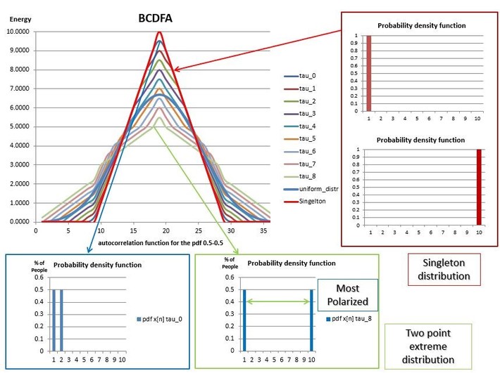
For instance, the figure above shows the BCDFA for a family of two -point distributions over ten categories. The curve tau_0 represents the nine distributions uniformly distributed over two contiguous categories (The histogram on the left bottom corner illustrates a member of this bimodal class of distributions). On the other hand, the curve tau_8 represent the two-point extreme distribution. Lastly, the red and light blue curves represent the singletons and uniform distribution, respectively. In this way, to quantify the distance between a pdf and the singleton distribution, it is only a matter of choosing an appropriate metric, which would assign larger values to distributions with more dispersed BCDFA than the singleton. For the definition and computation of the BCDFA see Appendix A3.
The selection of a measure to compare probability distribution is not a trivial matter and usually depends on the objectives. In this work, I propose the use of the Jensen-Shannon Divergence (Lin, 1991) . Since its definition is based on the BCDFA as opposed to density functions or CDF, is more regular than the variance, COV, IOV and LOV. In addition, unlike the other dispersion indices, this measure does not need to be normalized since is a bounded value in the unit interval. Another crucial characteristic of this metric is that it is infinite differentiable and its derivates are slowly decreasing than any power metric. A function with this characteristic is called tempered distribution or dual Schwartz functions (Stein & Shakarchi, 2003 p.134). Clearly, there are other functions that belong to this functional space (Taneja, 2001) (Jenssen, Principe, & Erologmus, 2006). However, the JSD is a well-known divergence and its square root is a metric (Endres & Schindelin, 2003). This last property will allow us to increase or reduce the magnitude of the divergence. Without loss of generality I call this class of functions, Divergence Index (DI).
Thank you for reading this technical post.
All the code required to compute the BCDF, ABCDF and DI is available on my GitHub account: