
The Data Science Method (DSM) – Pre-processing and Training Data Development
This is the fourth article in a series about how to take your data science projects to the next level by using a methodological approach similar to the scientific method coined the Data Science Method. This article is focused on the pre-processing of model development dataset and training data development. If you missed the previous article(s) in this series, you can go to the beginning here, or click on each step title below to read a specific step in the process.
The Data Science Method
- Problem Identification
- Data Collection, Organization, and Definitions
- Exploratory Data Analysis
- Pre-processing and Training Data Development
- Fit Models with Training Data Set
- Review Model Outcomes — Iterate over additional models as needed.
- Identify the Final Model
- Apply the Model to the Complete Data Set
- Review the Results — Share your findings
- Finalize Code and Documentation

Here are the general steps in pre-processing and training data development:
- Create dummy or indicator features for categorical variables
- Standardize the magnitude of numeric features
- Split into testing and training datasets
- Apply scaler to the testing set
- Create dummy or indicator features for categorical variables
Although some machine learning algorithms can interpret multi-level categorical variables, many machine learning models cannot handle categorical variables unless they are converted to dummy variables. I hate that term, ‘dummy variables’. Specifically, the variable is converted into a series of boolean variables for each level of a categorical feature. I first learned this concept as an indicator variable, as it indicates the presence or absence of something. For example, below we have the vehicle data set with three categorical columns; specifically, Manufacturer, Model, and vehicle type. We need to create an indicator column of each level of the manufacturer.
dfo=df.select_dtypes(include=[‘object’]) # select object type columns
df = pd.concat([df.drop(dfo, axis=1), pd.get_dummies(dfo)], axis=1)
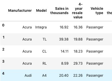
An original data frame with categorical features
First, we select all the columns that are categorical which are those with the data type = ‘object’, creating a data frame subset named ‘dfo’. Next, we concatenate the original data frame df while dropping those columns selected in the dfo, df.drop(dfo,axis=1), with the pandas.get_dummies(dfo)command, creating only indicator columns for the selected object data type columns and collating it with other numeric data frame columns.
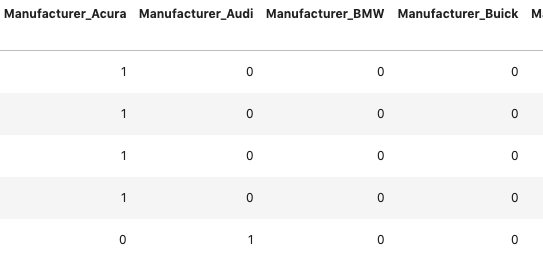
Dummies now added to the data frame with column name such as ‘Manufacturer_’
We perform this conversion regardless of the type of machine learning model we plan on developing because it allows a standardized data set for model development and further data manipulation should our planned approach not provide excellent results in the first pass. Pre-processing is the concept of standardizing your model development dataset.
2. Standardize the magnitude of numeric features
This is applied in situations where you have differences in the magnitude of numeric features. This would also be the juncture where other numeric translation would be applied to meet some scientific assumptions about the feature, such as accounting for atmospheric attenuation in satellite imagery data. However, you do not pass your dummy aka indicator features to the scaler; they do not need to be scaled as they as are boolean representations of categorical features.
Many machine learning algorithms objective functions are based on the assumption that the variables have mean of zero and have variance in the same order of magnitude of one, think L1 and L2 regularization. If the development features are not standardized then the larger magnitude features may dominate the objective function and further may spuriously reduce the impact of other features in the model.
Here is an example, the below data is also from the automobile sales dataset. You can see from the distribution plots for each feature that they vary in magnitude.
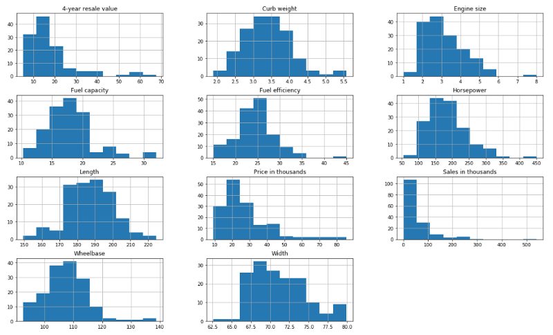
Numeric Features of differing magnitudes
When applying a scaler transformation we must save the scaler and apply the same transformation to the testing data subset. Therefore we apply it in two steps, first defining the scaler based on the mean and standard deviation of the training data and then applying that scaler to each the training and testing sets.
3. Split the data into training and testing subsets
Implementing a data subset approach with a train and test split with a 70/30 or 80/20 split is the general rule for an effective holdout test data for model validation. Review the code snippet and the other considerations below on splitting the model development data set into training and testing subsets.
4. Apply the standard scaler to the testing set
Before applying the scaler we split our dataset into training and testing dataset subsets so we can have a blind hold out sample in the testing set for model evaluation. It would also be appropriate to apply the standard data scaler to the entire data set and then split into test and train subsets afterward. It’s a matter of preference as to which comes first, just ensure the same adjustments applied to the training data are also carried through on the testing data.
from sklearn.model_selection import train_test_split
df=df.dropna()
X=df.drop([‘4-year resale value’], axis=1)
y=df[[‘4-year resale value’]]
X_train, X_test, y_train, y_test = train_test_split(X, y, test_size=0.25, random_state=1)
from sklearn import preprocessing
import numpy as np
scaler = preprocessing.StandardScaler().fit(X_train)
X_scaled=scaler.transform(X_train)
X_test_sc=scaler.transform(X_test)
Other Considerations in training data development
If you have time series data be sure to consider how to appropriately split your data into training and testing data for your optimal model outcome. Most likely you’re looking to forecast, and your testing subset should probably consist of the time most recent to the expected forecast or for the same period in a different year, or something logical for your particular data.
Additionally, if your data needs to be stratified during the testing and training data split, such as in our example if we considered European carmakers to be different strata then American carmakers we would have included the argument stratify=country in the train_test_split command.
In upcoming articles, I’ll cover machine learning model fitting and model review. Stay in touch by following me on Medium or Twitter. To receive updates about the Data Science Method or Data Science Professional Development Sign up here.
%20-Pre-processing%20and%20Training%20Data%20Development)