
Introduction
It is a well-known fact that neural networks can approximate the output of any continuous mathematical function, no matter how complicated it might be. Take for instance the function below:
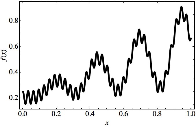
Though it has a pretty complicated shape, the theorems we will discuss shortly guarantee that one can build some neural network that can approximate f(x) as accurately as we want. Neural networks, therefore, display a type of universal behavior.
One of the reasons neural networks have received so much attention is that in addition to these rather remarkable universal properties, they possess many powerful algorithms for learning functions.
Universality and the underlying mathematics
This piece will give an informal overview of some of the fundamental mathematical results (theorems) underlying these approximation capabilities of artificial neural networks.
“Almost any process you can imagine can be thought of as function computation… [Examples include] naming a piece of music based on a short sample of the piece […], translating a Chinese text into English […], taking an mp4 movie file and generating a description of the plot of the movie, and a discussion of the quality of the acting.”
— Michael Nielsen
A motivation for using neural nets as approximators: Kolmogorov’s Theorem
In 1957, the Russian mathematician Andrey Kolmogorov (picture below) known for his contributions to a wide range of mathematical topics (such as probability theory, topology, turbulence, computational complexity, and many others), proved an important theorem about the representation of real functions of many variables. According to Kolmogorov’s theorem, multivariate functions can be expressed via a combination of sums and compositions of (a finite number of) univariate functions.

A little more formally, the theorem states that a continuous function f of real variables defined in the n-dimensional hypercube (with n ≥ 2) can be represented as follows:

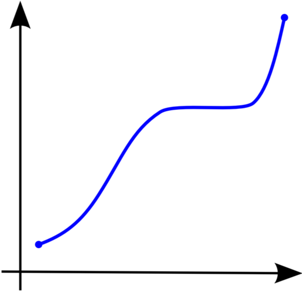
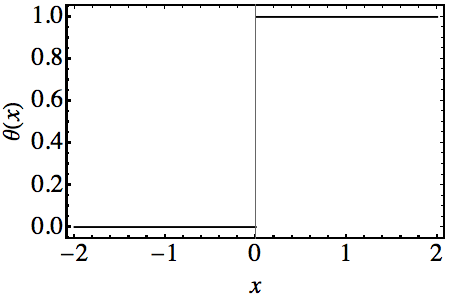
In this expression, the gs are univariate functions and the ϕs are continuous, entirely (monotonically) increasing functions (as shown in the figure below) that do not depend on the choice of f.
Universal Approximation Theorem (UAT)
The UAT states that feed-forward neural networks containing a single hidden layer with a finite number of nodes can be used to approximate any continuous function provided rather mild assumptions about the form of the activation function are satisfied. Now, since almost any process we can imagine can be described by some mathematical function, neural networks can, at least in principle, predict the outcome of nearly every process.
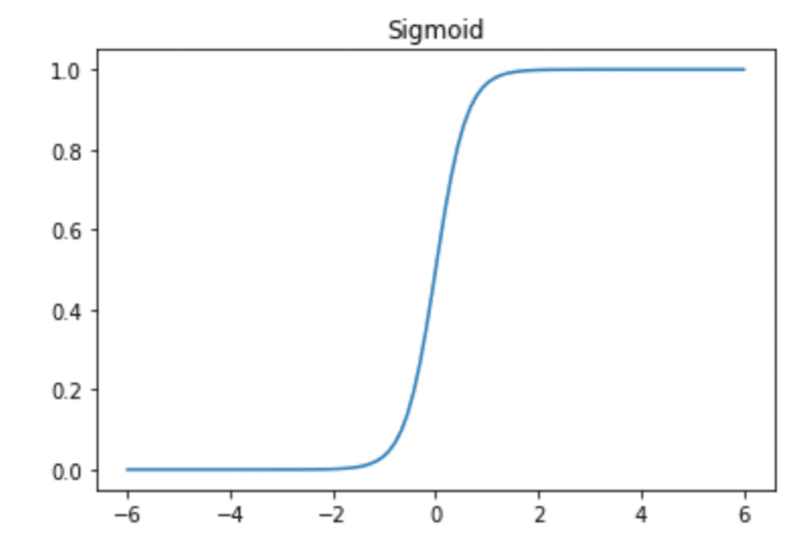
There are several rigorous proofs of the universality of feed-forward artificial neural nets using different activation functions. Let us, for the sake of brevity, restrict ourselves to the sigmoid function. Sigmoids are “S”-shaped and include as special cases the logistic function, the Gompertz curve, and the ogee curve.
Python code for the sigmoid
A quick Python code to build and plot a sigmoid function is:
import numpy as np
import matplotlib.pyplot as plt
%matplotlib inline
upper, lower = 6, -6
num = 100
def sigmoid_activation(x):
if x > upper:
return 1
 elif x < lower:
 return 0
 return 1/(1+np.exp(-x))
vals = [sigmoid_activation(x) for
x in np.linspace(lower, upper, num=num)]
plt.plot(np.linspace(lower,
 upper,
 num=num), vals);
 plt.title('Sigmoid');
George Cybenko’s Proof
The proof given by Cybenko (1989) is known for its elegance, simplicity, and conciseness. In his article, he proves the following statement. Let ϕ be any continuous function of the sigmoid type (see discussion above). Given any multivariate continuous function

inside a compact subset of the N-dimensional real space and any positive ϵ, there are vectors

(the weights), constants

(the bias terms) and

such that

for any x (the NN inputs) inside the compact subset, where the function G is given by:

Choosing the appropriate parameters, neural nets can be used to represent functions with a wide range of different forms.
An example using Python
To make these statements less abstract, let us build a simple Python code to illustrate what has been discussed until now. The following analysis is based on Michael Nielsen’s great online book and on the exceptional lectures byMatt Brems and Justin Pounders at the General Assembly Data Science Immersive (DSI).
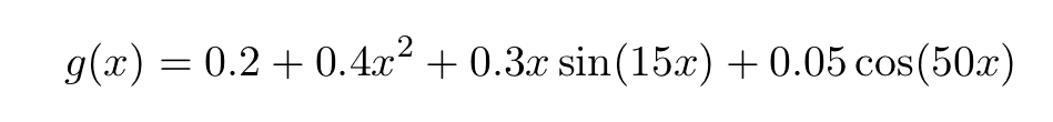
We will build a neural network to approximate the following simple function:
A few remarks are needed before diving into the code:
- To make the analysis more straightforward, I will work with a simple limit case of the sigmoid function. When the weights are extremely large, the sigmoid approaches the Heaviside step function. Since we will need to add contributions coming from several neurons, it is much more convenient to work with step functions instead of general sigmoids.
- In the limit where the sigmoid approaches the step function, we need only one parameter to describe it, namely, the point where the step occurs. The value of s can be shown to be equal to s=-b/w where b and w are the neuron’s bias and weight respectively.
- The neural network I will build will be a very simple one, with one input, one output, and one hidden layer. If the values of the weights corresponding to two hidden neurons are equal in absolute value and with opposite signs, their output becomes a “bump” with the height equal to the absolute value of the weights and width equal to the difference between the values of s of each neuron (see the figure below).
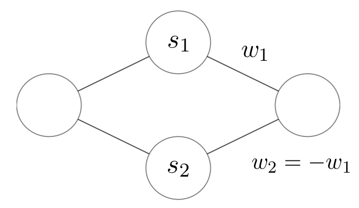
- We use the following notation since the absolute value of the weights is the height of the bump.

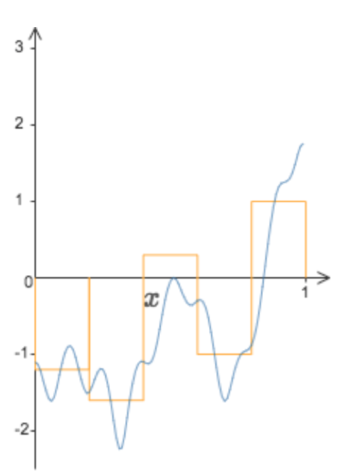
- Since we want to approximate g, the weighted output of the hidden layer must involve the inverse of the sigmoid. In fact, it must be equal to:

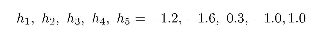
To reproduce this function, we choose the values of hs to be (see the corresponding figure below, taken from here):
The code
The code starts with the following definitions:
- We first import
inversefuncthat will need to build the inverse sigmoid function - We then choose a very large weight for the sigmoid for it to be similar to the Heaviside function (as just discussed).
- We choose the output activation to be the identity function
identify_activation - The role of the function is to recover the original (w,b) parametrization from s and w (recall that s is the step position).
- The architecture is set, and all the ws and bs are chosen. The elements of the array
weight_outputsare obtained from the values of the output weights given in the previous section.
from pynverse import inversefunc
w = 500
def identity_activation(x):
return(x)
def solve_for_bias(s, w=w):
return(-w * s)
steps = [0,.2,.2,.4,.4,.6,.6,.8,.8,1]
bias_hl = np.array([solve_for_bias(s) for s in steps])
weights_hl = np.array([w] * len(steps))
bias_output = 0
 weights_output =np.array([-1.2, 1.2, -1.6, 1.6,
 -.3, .3, -1])
 1, 1, 1, -1])
The final steps are:
- Writing a
Pythonfunction which I callednnthat builds and runs the network - Printing out the comparison between the approximation and the actual function.
def nn(input_value):

Z_hl = input_value * weights_hl + bias_hl
 activation_hl = np.array([sigmoid_activation(Z)
 for Z in Z_hl])
Z_output = np.sum(activation_hl * weights_output)
+ bias_output
activation_output = identity_activation(Z_output)

return activation_output
x_values = np.linspace(0,1,1000)
y_hat = [nn(x) for x in x_values]
def f(x):
return 0.2 + 0.4*(x**2) + 0.3*x*np.sin(15*x)+ 0.05*np.cos(50*x))
y = [f(x) for x in x_values]
inv_sigmoid = inversefunc(sigmoid_activation)
y_hat = [nn(x) for x in x_values]
y_invsig = [inv_sigmoid(i) for i in y]
_ = plt.plot(x_values, y_invsig)
 _ = plt.plot(x_values, y_hat)
 _ = plt.xlim((0,1))
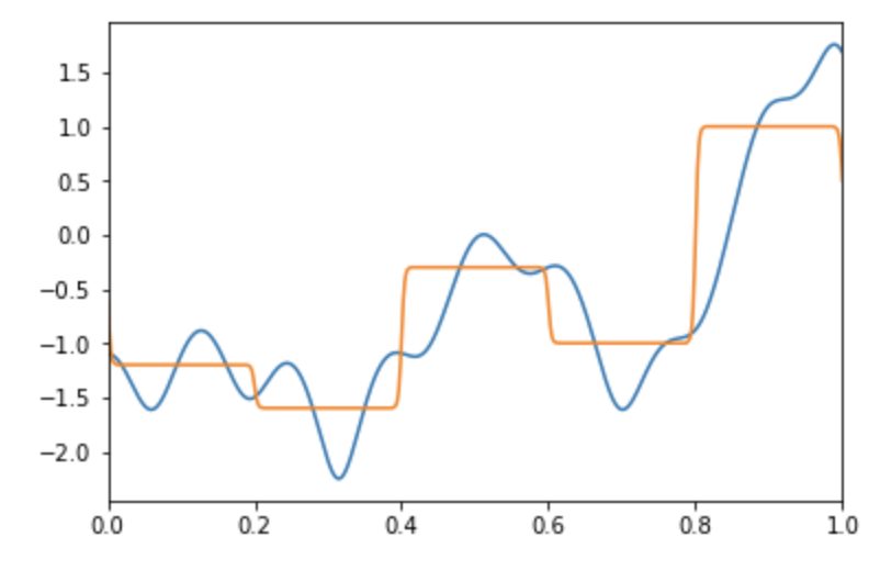
This approximation is far from ideal. However is it straightforward to improve it, for example, by increasing the number of nodes or the number of layers (but at the same time avoiding overfitting).
Conclusion
In this article, I described some basic mathematics underlying the universal properties of neural networks, and I showed a simple Python code that implements an approximation of a simple function.
Though the full code is already included in the article, my Github and my personal website www.marcotavora.me have (hopefully) some other interesting stuff both about data science and about physics.
Thanks for reading and see you soon!
By the way, constructive criticism and feedback are always welcome!
This article was originally published on Towards Data Science.
)